spikingjelly.visualizing package#
- spikingjelly.visualizing.plot_1d_spikes(spikes, title, xlabel, ylabel, int_x_ticks=True, int_y_ticks=True, plot_firing_rate=True, firing_rate_map_title='firing rate', figsize=(12, 8), dpi=200)[源代码]#
-
中文
画出 N 个时长为 T 的脉冲数据。可以用来画 N 个神经元在 T 个时刻的脉冲发放情况。
- 参数:
spikes (Union[np.ndarray, Tensor]) -- shape=[T, N] 的数组,元素只能为 0 或 1,表示 N 个时长为 T 的脉冲数据。 支持
np.ndarray或torch.Tensortitle (str) -- 图的标题
xlabel (str) -- x轴标签
ylabel (str) -- y轴标签
int_x_ticks (bool) -- x轴是否只显示整数刻度
int_y_ticks (bool) -- y轴是否只显示整数刻度
plot_firing_rate (bool) -- 是否画出各脉冲发放频率
firing_rate_map_title (str) -- 脉冲频率发放图的标题
dpi (int) -- 绘图 dpi
- 返回:
(fig, ax)元组,其中ax是脉冲图的 axes- 返回类型:
Tuple[matplotlib.figure.Figure, matplotlib.axes.Axes]
- 抛出:
ValueError -- 当
spikes不是二维数组时
English
Plot spike data for N neurons over T time steps.
- 参数:
spikes (Union[np.ndarray, Tensor]) -- Array of shape=[T, N] with values in {0, 1}, representing spike trains of N neurons over T steps. Accepts
np.ndarrayortorch.Tensor.title (str) -- Title of the plot.
xlabel (str) -- Label of the x-axis.
ylabel (str) -- Label of the y-axis.
int_x_ticks (bool) -- Whether to show only integer ticks on the x-axis.
int_y_ticks (bool) -- Whether to show only integer ticks on the y-axis.
plot_firing_rate (bool) -- Whether to draw a firing rate bar beside the spike plot.
firing_rate_map_title (str) -- Title of the firing rate subplot.
dpi (int) -- Dots per inch.
- 返回:
(fig, ax)tuple whereaxis the spike plot axes.- 返回类型:
Tuple[matplotlib.figure.Figure, matplotlib.axes.Axes]
- 抛出:
ValueError -- If
spikesis not 2-dimensional.
代码示例 | Example
import torch
from spikingjelly.activation_based import neuron
from spikingjelly import visualizing
from matplotlib import pyplot as plt

lif = neuron.LIFNode(tau=100.0)
x = torch.rand(size=[32]) * 4
T = 50
s_list = []
for t in range(T):
    s_list.append(lif(x).unsqueeze(0))

s_list = torch.cat(s_list)

fig, ax = visualizing.plot_1d_spikes(
    spikes=s_list,
    title="Spikes",
    xlabel="Simulating Step",
    ylabel="Neuron Index",
    dpi=200,
)
plt.show()

- spikingjelly.visualizing.plot_2d_bar_in_3d(array, title, xlabel, ylabel, zlabel, int_x_ticks=True, int_y_ticks=True, int_z_ticks=False, dpi=200)[源代码]#
-
中文
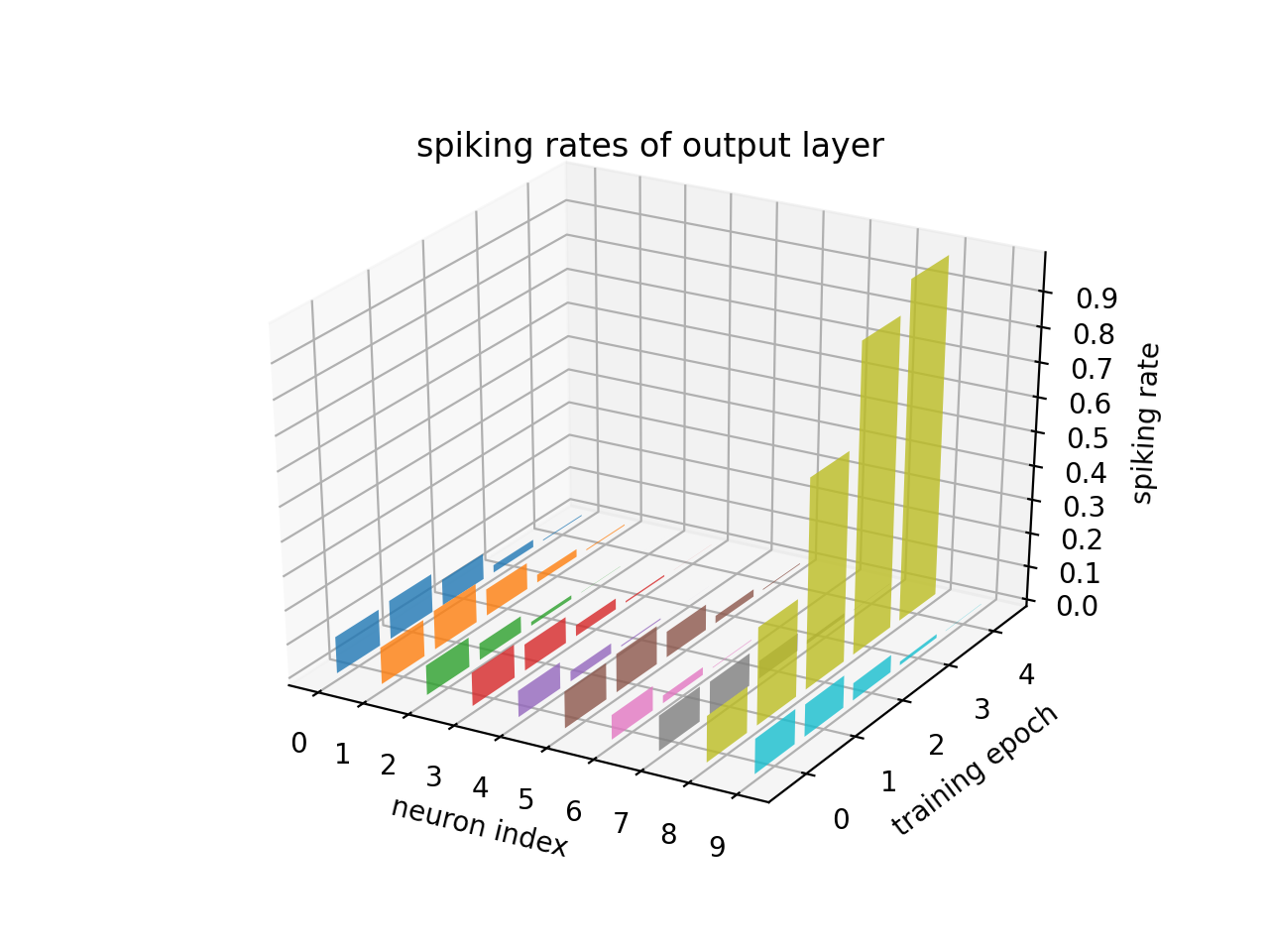
将 shape=[T, N] 的数组绘制为三维柱状图。可以用来绘制多个神经元的脉冲发放频率随时间的变化情况。
- 参数:
- 返回:
(fig, ax)元组- 返回类型:
Tuple[matplotlib.figure.Figure, matplotlib.axes.Axes]
- 抛出:
ValueError -- 当
array不是二维数组时
English
Plot a shape=[T, N] array as a 3D bar chart. Useful for visualizing firing rates of multiple neurons changing over time.
- 参数:
array (Union[np.ndarray, Tensor]) -- Array of shape=[T, N]. Accepts
np.ndarrayortorch.Tensor.title (str) -- Title of the plot.
xlabel (str) -- Label of the x-axis.
ylabel (str) -- Label of the y-axis.
zlabel (str) -- Label of the z-axis.
int_x_ticks (bool) -- Whether to show only integer ticks on the x-axis.
int_y_ticks (bool) -- Whether to show only integer ticks on the y-axis.
int_z_ticks (bool) -- Whether to show only integer ticks on the z-axis.
dpi (int) -- Dots per inch.
- 返回:
(fig, ax)tuple.- 返回类型:
Tuple[matplotlib.figure.Figure, matplotlib.axes.Axes]
- 抛出:
ValueError -- If
arrayis not 2-dimensional.
代码示例 | Example
import torch
from spikingjelly import visualizing
from matplotlib import pyplot as plt

Epochs = 5
N = 10
firing_rate = torch.zeros(Epochs, N)
init_firing_rate = torch.rand(size=[N])
for i in range(Epochs):
    firing_rate[i] = torch.softmax(init_firing_rate * (i + 1) ** 2, dim=0)
fig, ax = visualizing.plot_2d_bar_in_3d(
    firing_rate,
    title="spiking rates of output layer",
    xlabel="neuron index",
    ylabel="training epoch",
    zlabel="spiking rate",
)
plt.show()
- spikingjelly.visualizing.plot_2d_feature_map(x3d, nrows, ncols, space, title, figsize=(12, 8), dpi=200)[源代码]#
-
中文
将 C 个尺寸为 W x H 的矩阵全部画出,排列成 nrows 行 ncols 列。这样的矩阵一般来源于卷积层后脉冲神经元的输出。
- 参数:
- 返回:
(fig, ax)元组- 返回类型:
Tuple[matplotlib.figure.Figure, matplotlib.axes.Axes]
- 抛出:
ValueError -- 当
x3d不是三维数组时,或nrows * ncols != C时
English
Plot C matrices of size W x H arranged in a grid of
nrowsrows andncolscolumns. These matrices typically come from the output of convolutional spiking layers.- 参数:
x3d (Union[np.ndarray, Tensor]) -- Array of shape=[C, W, H]. Accepts
np.ndarrayortorch.Tensor.nrows (int) -- Number of rows in the grid.
ncols (int) -- Number of columns in the grid.
space (int) -- Gap (in pixels) between adjacent matrices.
title (str) -- Title of the plot.
dpi (int) -- Dots per inch.
- 返回:
(fig, ax)tuple.- 返回类型:
Tuple[matplotlib.figure.Figure, matplotlib.axes.Axes]
- 抛出:
ValueError -- If
x3dis not 3-dimensional, ornrows * ncols != C.
代码示例 | Example
from spikingjelly import visualizing
import numpy as np
from matplotlib import pyplot as plt

C = 48
W = 8
H = 8
spikes = (np.random.rand(C, W, H) > 0.8).astype(float)
fig, ax = visualizing.plot_2d_feature_map(
    x3d=spikes, nrows=6, ncols=8, space=2, title="Spiking Feature Maps", dpi=200
)
plt.show()

- spikingjelly.visualizing.plot_2d_heatmap(array, title, xlabel, ylabel, int_x_ticks=True, int_y_ticks=True, plot_colorbar=True, colorbar_y_label='magnitude', x_max=None, figsize=(12, 8), dpi=200)[源代码]#
-
中文
绘制一张二维热力图。可以用来绘制多个神经元在不同时刻的电压。
- 参数:
array (Union[np.ndarray, Tensor]) -- shape=[T, N]的数组,支持
np.ndarray或torch.Tensortitle (str) -- 热力图标题
xlabel (str) -- x轴标签
ylabel (str) -- y轴标签
int_x_ticks (bool) -- x轴是否只显示整数刻度
int_y_ticks (bool) -- y轴是否只显示整数刻度
plot_colorbar (bool) -- 是否画出颜色-数值对应关系的 colorbar
colorbar_y_label (str) -- colorbar 的 y 轴标签
x_max (Optional[float]) -- 横轴最大刻度。若为
None,则为array.shape[1]dpi (int) -- 绘图 dpi
- 返回:
(fig, ax)元组- 返回类型:
Tuple[matplotlib.figure.Figure, matplotlib.axes.Axes]
- 抛出:
ValueError -- 当
array不是二维数组时
English
Plot a 2D heatmap. Useful for visualizing membrane potentials of multiple neurons over time.
- 参数:
array (Union[np.ndarray, Tensor]) -- Array of shape=[T, N]. Accepts
np.ndarrayortorch.Tensor.title (str) -- Title of the heatmap.
xlabel (str) -- Label of the x-axis.
ylabel (str) -- Label of the y-axis.
int_x_ticks (bool) -- Whether to show only integer ticks on the x-axis.
int_y_ticks (bool) -- Whether to show only integer ticks on the y-axis.
plot_colorbar (bool) -- Whether to draw a colorbar showing the color-value mapping.
colorbar_y_label (str) -- Label of the colorbar y-axis.
x_max (Optional[float]) -- Maximum tick on the x-axis. If
None, defaults toarray.shape[1].dpi (int) -- Dots per inch.
- 返回:
(fig, ax)tuple.- 返回类型:
Tuple[matplotlib.figure.Figure, matplotlib.axes.Axes]
- 抛出:
ValueError -- If
arrayis not 2-dimensional.
代码示例 | Example
import torch
from spikingjelly.activation_based import neuron
from spikingjelly import visualizing
from matplotlib import pyplot as plt

lif = neuron.LIFNode(tau=100.0)
x = torch.rand(size=[32]) * 4
T = 50
s_list = []
v_list = []
for t in range(T):
    s_list.append(lif(x).unsqueeze(0))
    v_list.append(lif.v.unsqueeze(0))

s_list = torch.cat(s_list)
v_list = torch.cat(v_list)

fig, ax = visualizing.plot_2d_heatmap(
    array=v_list,
    title="Membrane Potentials",
    xlabel="Simulating Step",
    ylabel="Neuron Index",
    int_x_ticks=True,
    x_max=T,
    dpi=200,
)
plt.show()

- spikingjelly.visualizing.plot_one_neuron_v_s(v, s, v_threshold=1.0, v_reset=0.0, title='$V[t]$ and $S[t]$ of the neuron', figsize=(12, 8), dpi=200)[源代码]#
-
中文
绘制单个神经元的电压、脉冲随着时间的变化情况。
- 参数:
- 返回:
(fig, ax_voltage, ax_spike)三元组- 返回类型:
Tuple[matplotlib.figure.Figure, matplotlib.axes.Axes, matplotlib.axes.Axes]
- 抛出:
ValueError -- 当
v或s不是一维数组时
English
Plot the membrane voltage and spike train of a single neuron over time.
- 参数:
v (Union[np.ndarray, Tensor]) -- Array of shape=[T] storing membrane voltage at each time step. Accepts
np.ndarrayortorch.Tensor.s (Union[np.ndarray, Tensor]) -- Array of shape=[T] storing spikes emitted at each time step. Accepts
np.ndarrayortorch.Tensor.v_threshold (float) -- Threshold voltage of the neuron.
v_reset (Optional[float]) -- Reset voltage of the neuron. Can be
None.title (str) -- Title of the plot.
dpi (int) -- Dots per inch.
- 返回:
(fig, ax_voltage, ax_spike)triple.- 返回类型:
Tuple[matplotlib.figure.Figure, matplotlib.axes.Axes, matplotlib.axes.Axes]
- 抛出:
ValueError -- If
vorsis not 1-dimensional.
代码示例 | Example
import torch
from spikingjelly.activation_based import neuron
from spikingjelly import visualizing
from matplotlib import pyplot as plt

lif = neuron.LIFNode(tau=100.0)
x = torch.Tensor([2.0])
T = 150
s_list = []
v_list = []
for t in range(T):
    s_list.append(lif(x))
    v_list.append(lif.v)
fig, ax_v, ax_s = visualizing.plot_one_neuron_v_s(
    v_list, s_list, v_threshold=lif.v_threshold, v_reset=lif.v_reset
)
plt.show()
