Clock_driven
Author: fangwei123456, lucifer2859
This tutorial focuses on spikingjelly.clock_driven, introducing the clock-driven simulation method, the concept of surrogate gradient method, and the use of differentiable spiking neurons.
The surrogate gradient method is a new method emerging in recent years. For more information about this method, please refer to the following overview:
Neftci E, Mostafa H, Zenke F, et al. Surrogate Gradient Learning in Spiking Neural Networks: Bringing the Power of Gradient-based optimization to spiking neural networks[J]. IEEE Signal Processing Magazine, 2019, 36(6): 51-63.
The download address for this article can be found at arXiv .
SNN Compared with RNN
The neuron in SNN can be regarded as a kind of RNN, and its input is the voltage increment (or the product of current and membrane resistance, but for convenience, clock_driven.neuron uses voltage increment). The hidden state is the membrane voltage, and the output is a spike. Such spiking neurons are Markovian: the output at the current time is only related to the input at the current time and the state of the neuron itself.
You can use three discrete equations —— Charge, Discharge, Reset —— to describe any discrete spiking neuron:
where \(V(t)\) is the membrane voltage of the neuron; \(X(t)\) is an external source input, such as voltage increment; \(H(t)\) is the hidden state of the neuron, which can be understood as the instant before the neuron has not fired a spike; \(f(V(t-1), X(t))\) is the state update equation of the neuron. Different neurons differ in the update equation.
For example, for a LIF neuron, we describe the differential equation of its dynamics below a threshold, and the corresponding difference equation are:
The corresponding Charge equation is
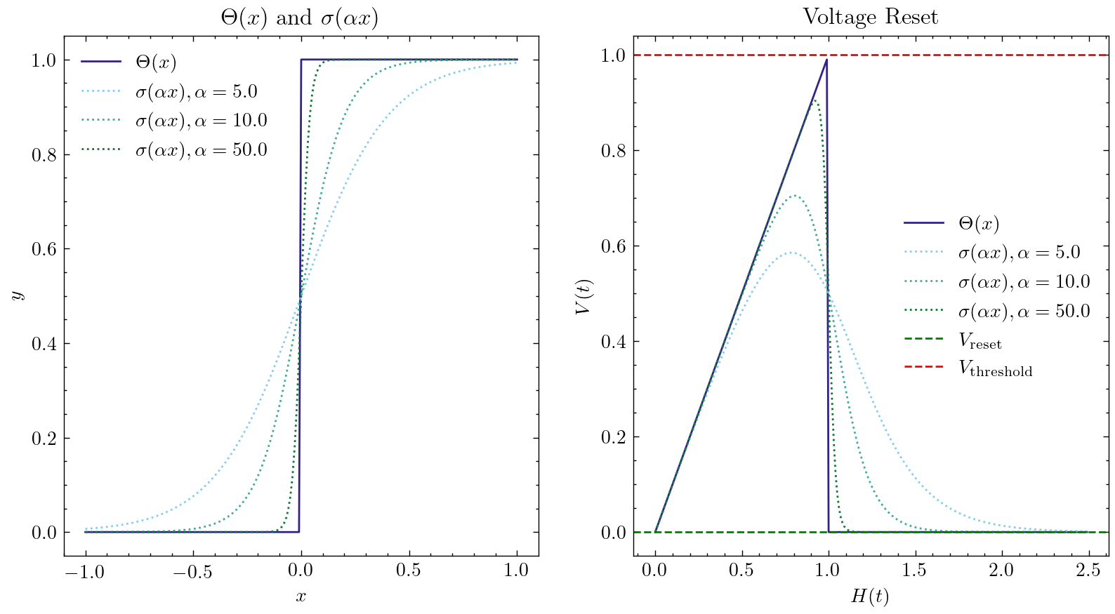
In the Discharge equation, \(S(t)\) is a spike fired by a neuron, \(g(x)=\Theta(x)\) is a step function. RNN is used to call it a gating function. In SNN, it is called a spiking function. The output of the spiking function is only 0 or 1, which can represent the firing process of spike, defined as
Reset means the reset process of the voltage: when a spike is fired, the voltage is reset to \(V_{reset}\); If no spike is fired, the voltage remains unchanged.
Surrogate Gradient Method
RNN uses differentiable gating functions, such as the tanh function. Obviously, the spiking function of SNN \(g(x)=\Theta(x)\) is not differentiable, which leads to the fact that SNN is very similar to RNN to a certain extent, but it cannot be trained by gradient descent and back-propagation. We can use a gating function that is very similar to \(g(x)=\Theta(x)\) , but differentiable \(\sigma(x)\) to replace it.
The core idea of this method is: when forwarding, using \(g(x)=\Theta(x)\), the output of the neuron is discrete 0 and 1, and our network is still SNN; When back-propagation, the gradient of the surrogate gradient function \(g'(x)=\sigma'(x)\) is used to replace the gradient of the spiking function. The most common surrogate gradient function is the sigmoid function \(\sigma(\alpha x)=\frac{1}{1 + exp(-\alpha x)}\). \(\alpha\) can control the smoothness of the function. The function with larger \(\alpha\) will be closer to \(\Theta(x)\). But when it gets closer to \(x=0\), the gradient will be more likely to explode. And when it gets farther to \(x=0\), the gradient will be more likely to disappear. This makes the network more difficult to train. The following figure shows the shape of the surrogate gradient function and the corresponding Reset equation for different \(\alpha\):
The default surrogate gradient function is clock_driven.surrogate.Sigmoid(), clock_driven.surrogate also provides other optional approximate gating functions.
The surrogate gradient function is one of the parameters of the neuron constructor in clock_driven.neuron:
class BaseNode(base.MemoryModule):
    def __init__(self, v_threshold: float = 1., v_reset: float = 0.,
                surrogate_function: Callable = surrogate.Sigmoid(), detach_reset: bool = False):
        """
        :param v_threshold: threshold voltage of neurons
        :type v_threshold: float

        :param v_reset: reset voltage of neurons. If not ``None``, voltage of neurons that just fired spikes will be set to
            ``v_reset``. If ``None``, voltage of neurons that just fired spikes will subtract ``v_threshold``
        :type v_reset: float

        :param surrogate_function: surrogate function for replacing gradient of spiking functions during back-propagation
        :type surrogate_function: Callable

        :param detach_reset: whether detach the computation graph of reset
        :type detach_reset: bool

        This class is the base class of differentiable spiking neurons.
        """
If you want to customize the new approximate gating function, you can refer to the code in clock_driven.surrogate. Usually we define it as torch.autograd.Function, and then encapsulate it into a subclass of torch.nn.Module.
Embed Spiking Neurons into Deep Networks
After solving the differential problem of spiking neurons, our spiking neurons can be embedded into any network built using PyTorch like an activation function, making the network an SNN. Some classic neurons have been implemented in clock_driven.neuron, which can easily build various networks, such as a simple fully connected network:
net = nn.Sequential(
        nn.Linear(100, 10, bias=False),
        neuron.LIFNode(tau=100.0, v_threshold=1.0, v_reset=5.0)
        )
Example: MNIST classification using a single-layer fully connected network
Now we use the LIF neurons in clock_driven.neuron to build a one-layer fully connected network to classify the MNIST dataset.
Firstly, we confirm hyperparameters we needed:
parser.add_argument('--device', default='cuda:0', help='Device, e.g., "cpu" or "cuda:0"')

parser.add_argument('--dataset-dir', default='./', help='Root directory for saving MNIST dataset, e.g., "./"')
parser.add_argument('--log-dir', default='./', help='Root directory for saving tensorboard logs, e.g., "./"')
parser.add_argument('--model-output-dir', default='./', help='Model directory for saving, e.g., "./"')

parser.add_argument('-b', '--batch-size', default=64, type=int, help='Batch size, e.g., "64"')
parser.add_argument('-T', '--timesteps', default=100, type=int, dest='T', help='Simulating timesteps, e.g., "100"')
parser.add_argument('--lr', '--learning-rate', default=1e-3, type=float, metavar='LR', help='Learning rate, e.g., "1e-3": ', dest='lr')
parser.add_argument('--tau', default=2.0, type=float, help='Membrane time constant, tau, for LIF neurons, e.g., "100.0"')
parser.add_argument('-N', '--epoch', default=100, type=int, help='Training epoch, e.g., "100"')
Initialize the DataLoader:
# Initialize the DataLoader
train_dataset = torchvision.datasets.MNIST(
    root=dataset_dir,
    train=True,
    transform=torchvision.transforms.ToTensor(),
    download=True
)
test_dataset = torchvision.datasets.MNIST(
    root=dataset_dir,
    train=False,
    transform=torchvision.transforms.ToTensor(),
    download=True
)

train_data_loader = data.DataLoader(
    dataset=train_dataset,
    batch_size=batch_size,
    shuffle=True,
    drop_last=True
)
test_data_loader = data.DataLoader(
    dataset=test_dataset,
    batch_size=batch_size,
    shuffle=False,
    drop_last=False
)
Define our network structure:
# Define SNN
net = nn.Sequential(
    nn.Flatten(),
    nn.Linear(28 * 28, 10, bias=False),
    neuron.LIFNode(tau=tau)
)
net = net.to(device)
Initialize the optimizer and encoder (we use a Poisson encoder to encode the MNIST image into spike trains):
# Use Adam optimizer
optimizer = torch.optim.Adam(net.parameters(), lr=lr)
# Use Poisson encoder
encoder = encoding.PoissonEncoder()
The training of the network is simple. Run the network for T time steps to accumulate the output spikes of 10 neurons in the output layer to obtain the number of spikes fired by the output layer out_spikes_counter; Use the firing times of the spike divided by the simulation duration to get the firing frequency of the output layer out_spikes_counter_frequency = out_spikes_counter / T. We hope that when the real category of the input image is i, the i-th neuron in the output layer has the maximum activation degree, while the other neurons remain silent. Therefore, the loss function is naturally defined as the firing frequency of the output layer out_spikes_counter_frequency and the cross-entropy of label_one_hot obtained after one-hot encoding with the real category, or MSE. We use MSE because the experiment found that MSE is better. In particular, note that SNN is a stateful, or memorized network. So before entering new data, you must reset the state of the network. This can be done by calling clock_driven.functional.reset_net(net) to fulfill. The training code is as follows:
print("Epoch {}:".format(epoch))
print("Training...")
train_correct_sum = 0
train_sum = 0
net.train()
for img, label in tqdm(train_data_loader):
    img = img.to(device)
    label = label.to(device)
    label_one_hot = F.one_hot(label, 10).float()

    optimizer.zero_grad()

    # Run for T durations, out_spikes_counter is a tensor with shape=[batch_size, 10]
    # Record the number of spikes delivered by the 10 neurons in the output layer during the entire simulation duration
    for t in range(T):
        if t == 0:
            out_spikes_counter = net(encoder(img).float())
        else:
            out_spikes_counter += net(encoder(img).float())

    # out_spikes_counter / T # Obtain the firing frequency of 10 neurons in the output layer within the simulation duration
    out_spikes_counter_frequency = out_spikes_counter / T

    # The loss function is the firing frequency of the neurons in the output layer, and the MSE of the real class
    # Such a loss function causes that when the category i is input, the firing frequency of the i-th neuron in the output layer approaches 1, while the firing frequency of other neurons approaches 0.
    loss = F.mse_loss(out_spikes_counter_frequency, label_one_hot)
    loss.backward()
    optimizer.step()
    # After optimizing the parameters once, the state of the network needs to be reset, because the SNN neurons have "memory"
    functional.reset_net(net)

    # Calculation of accuracy. The index of the neuron with max frequency in the output layer is the classification result.
    train_correct_sum += (out_spikes_counter_frequency.max(1)[1] == label.to(device)).float().sum().item()
    train_sum += label.numel()

    train_batch_accuracy = (out_spikes_counter_frequency.max(1)[1] == label.to(device)).float().mean().item()
    writer.add_scalar('train_batch_accuracy', train_batch_accuracy, train_times)
    train_accs.append(train_batch_accuracy)

    train_times += 1
train_accuracy = train_correct_sum / train_sum
The test code is simpler than the training code:
print("Testing...")
net.eval()
with torch.no_grad():
    # Each time through the entire data set, test once on the test set
    test_sum = 0
    correct_sum = 0
    for img, label in tqdm(test_data_loader):
        img = img.to(device)
        for t in range(T):
            if t == 0:
                out_spikes_counter = net(encoder(img).float())
            else:
                out_spikes_counter += net(encoder(img).float())

        correct_sum += (out_spikes_counter.max(1)[1] == label.to(device)).float().sum().item()
        test_sum += label.numel()
        functional.reset_net(net)
    test_accuracy = correct_sum / test_sum
    writer.add_scalar('test_accuracy', test_accuracy, epoch)
    test_accs.append(test_accuracy)
    max_test_accuracy = max(max_test_accuracy, test_accuracy)
print("Epoch {}: train_acc={}, test_acc={}, max_test_acc={}, train_times={}".format(epoch, train_accuracy, test_accuracy, max_test_accuracy, train_times))
print()
The complete code is located at clock_driven.examples.lif_fc_mnist.py. In the code, we also use Tensorboard to save the training log.
Here are the (hyper)parameters you can configure:
$ python <PATH>/lif_fc_mnist.py --help
usage: lif_fc_mnist.py [-h] [--device DEVICE] [--dataset-dir DATASET_DIR] [--log-dir LOG_DIR] [--model-output-dir MODEL_OUTPUT_DIR] [-b BATCH_SIZE] [-T T] [--lr LR] [--tau TAU] [-N EPOCH]

spikingjelly LIF MNIST Training

optional arguments:
-h, --help            show this help message and exit
--device DEVICE       运行的设备,例如“cpu”或“cuda:0” Device, e.g., "cpu" or "cuda:0"
--dataset-dir DATASET_DIR
                        保存MNIST数据集的位置,例如“./” Root directory for saving MNIST dataset, e.g., "./"
--log-dir LOG_DIR     保存tensorboard日志文件的位置,例如“./” Root directory for saving tensorboard logs, e.g., "./"
--model-output-dir MODEL_OUTPUT_DIR
                        模型保存路径,例如“./” Model directory for saving, e.g., "./"
-b BATCH_SIZE, --batch-size BATCH_SIZE
                        Batch 大小,例如“64” Batch size, e.g., "64"
-T T, --timesteps T   仿真时长,例如“100” Simulating timesteps, e.g., "100"
--lr LR, --learning-rate LR
                        学习率,例如“1e-3” Learning rate, e.g., "1e-3":
--tau TAU             LIF神经元的时间常数tau,例如“100.0” Membrane time constant, tau, for LIF neurons, e.g., "100.0"
-N EPOCH, --epoch EPOCH
                        训练epoch,例如“100” Training epoch, e.g., "100"
You can also run it directly on the Python command line:
$ python
>>> import spikingjelly.clock_driven.examples.lif_fc_mnist as lif_fc_mnist
>>> lif_fc_mnist.main()
########## Configurations ##########
device=cuda:0
dataset_dir=./
log_dir=./
model_output_dir=./
batch_size=64
T=100
lr=0.001
tau=2.0
epoch=100
####################################
Epoch 0:
Training...
100%|█████████████████████████████████████████████████████████████████████████████████████████████████████████████████████████████████████████████████████████████████████████████████████████████████████████████████| 937/937 [01:26<00:00, 10.89it/s]
Testing...
100%|█████████████████████████████████████████████████████████████████████████████████████████████████████████████████████████████████████████████████████████████████████████████████████████████████████████████████| 157/157 [00:05<00:00, 28.79it/s]
Epoch 0: train_acc = 0.8641775613660619, test_acc=0.9071, max_test_acc=0.9071, train_times=937
Save and load model:
# Save model
torch.save(net, model_output_dir + "/lif_snn_mnist.ckpt")
# Load model
# net = torch.load(model_output_dir + "/lif_snn_mnist.ckpt")
It should be noted that the amount of memory required to train such an SNN is linearly related to the simulation time T. A longer T is equivalent to using a smaller simulation step size and training is more “fine”, however, the training effect is not necessarily better. So if T is too large, the SNN will become a very deep network after being expanded in time, and the gradient is easy to decay or explode. Since we use a Poisson encoder, a larger T is required.
Our model, training 100 epochs on Tesla K80, takes about 75 minutes. The changes in the accuracy of each batch and the accuracy of the test set during training are as follows:
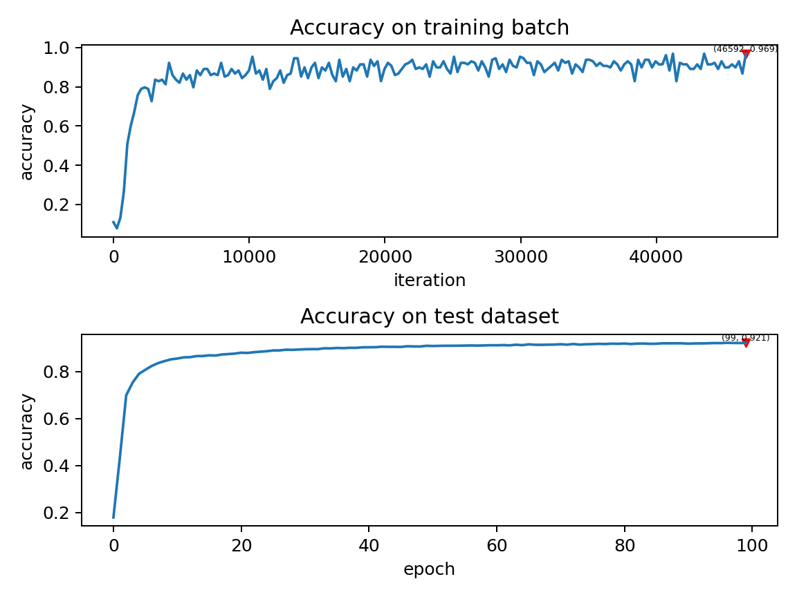
The final test set accuracy rate is about 92%, which is not a very high accuracy rate, because we use a very simple network structure and Poisson encoder. We can completely remove the Poisson encoder and send the image directly to the SNN. In this case, the first layer of LIF neurons can be regarded as an encoder.