Recurrent Connections and Stateful Synapses
Author: fangwei123456
Recurrent Connections
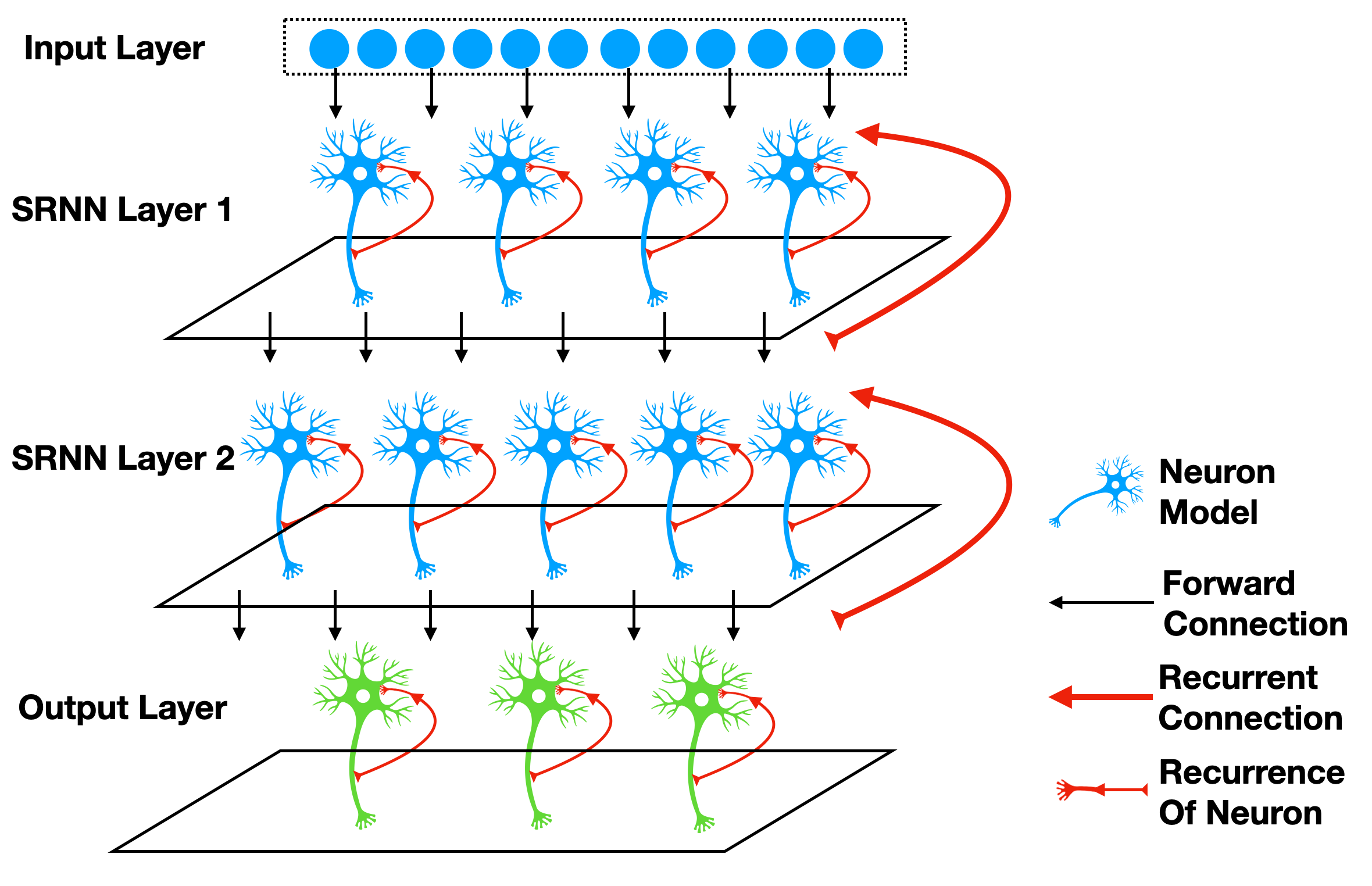
The recurrent connections connect a module’s outputs to its inputs. For example, 1 uses a SRNN(recurrent networks of spiking neurons), which is shown in the following figure:
It is easy to use SpikingJelly to implement the recurrent module. Considering a simple case that we add a connection to make
the neuron’s outputs \(s[t]\) at time-step \(t\) can add with external inputs \(x[t+1]\) at time-step \(t+1\).
It can be implemented by spikingjelly.clock_driven.layer.ElementWiseRecurrentContainer. ElementWiseRecurrentContainer
is a container that add a recurrent connection to the contained sub_module. The connection is a user-defined element-wise
function \(z=f(x, y)\). Denote the inputs and outputs of sub_module as \(i[t]\) and \(y[t]\) (Note that
\(y[t]\) is also the outputs of this module), and the inputs of this module as \(x[t]\), then
where \(f\) is the user-defined element-wise function. We set \(y[-1] = 0\).
Let us use ElementWiseRecurrentContainer to contain a IF neuron, and set the element-wise function as add:
We use soft reset, and give the inputs as \(x[t]=[1.5, 0, ..., 0]\):
T = 8
def element_wise_add(x, y):
    return x + y
net = ElementWiseRecurrentContainer(neuron.IFNode(v_reset=None), element_wise_add)
print(net)
x = torch.zeros([T])
x[0] = 1.5
for t in range(T):
    print(t, f'x[t]={x[t]}, s[t]={net(x[t])}')

functional.reset_net(net)
The outputs are:
ElementWiseRecurrentContainer(
  element-wise function=<function element_wise_add at 0x000001FE0F7968B0>
  (sub_module): IFNode(
    v_threshold=1.0, v_reset=None, detach_reset=False
    (surrogate_function): Sigmoid(alpha=1.0, spiking=True)
  )
)
0 x[t]=1.5, s[t]=1.0
1 x[t]=0.0, s[t]=1.0
2 x[t]=0.0, s[t]=1.0
3 x[t]=0.0, s[t]=1.0
4 x[t]=0.0, s[t]=1.0
5 x[t]=0.0, s[t]=1.0
6 x[t]=0.0, s[t]=1.0
7 x[t]=0.0, s[t]=1.0
We can find that due to the recurrent connection, even if \(x[t]=0\) when \(t \ge 1\), the neuron can still fire because its output spike is fed back as input.
We can use spikingjelly.clock_driven.layer.LinearRecurrentContainer to implement a more complex recurrent connections.
Stateful Synapses
There are many papers using stateful synapses, e.g., 2 3. We can put spikingjelly.clock_driven.layer.SynapseFilter after a stateless synapse to get the stateful synapse:
stateful_conv = nn.Sequential(
    nn.Conv2d(3, 16, kernel_size=3, padding=1, stride=1),
    SynapseFilter(tau=100, learnable=True)
)
Ablation Study On Sequential FashionMNIST
Now we do a smple exmperiment on Sequential FashionMNIST to check whether recurrent connections and stateful synapses can promote the network’s temporal information fitting ability. Sequential FashionMNIST is using FashionMNIST as input row-by-row
or column-by-column, rather than the whole image. Consequentially, the network classify Sequential FashionMNIST correctly
only when it can learn long-term dependencies. We will feed the image column-by-column, which is same with reading texts from left to right. Here is the example:

The following gif shows the column being read:

First, let us import packages:
import torch
import torch.nn as nn
import torch.nn.functional as F
import torchvision.datasets
from spikingjelly.clock_driven.model import train_classify
from spikingjelly.clock_driven import neuron, surrogate, layer
from spikingjelly.clock_driven.functional import seq_to_ann_forward
from torchvision import transforms
import os, argparse

try:
    import cupy
    backend = 'cupy'
except ImportError:
    backend = 'torch'
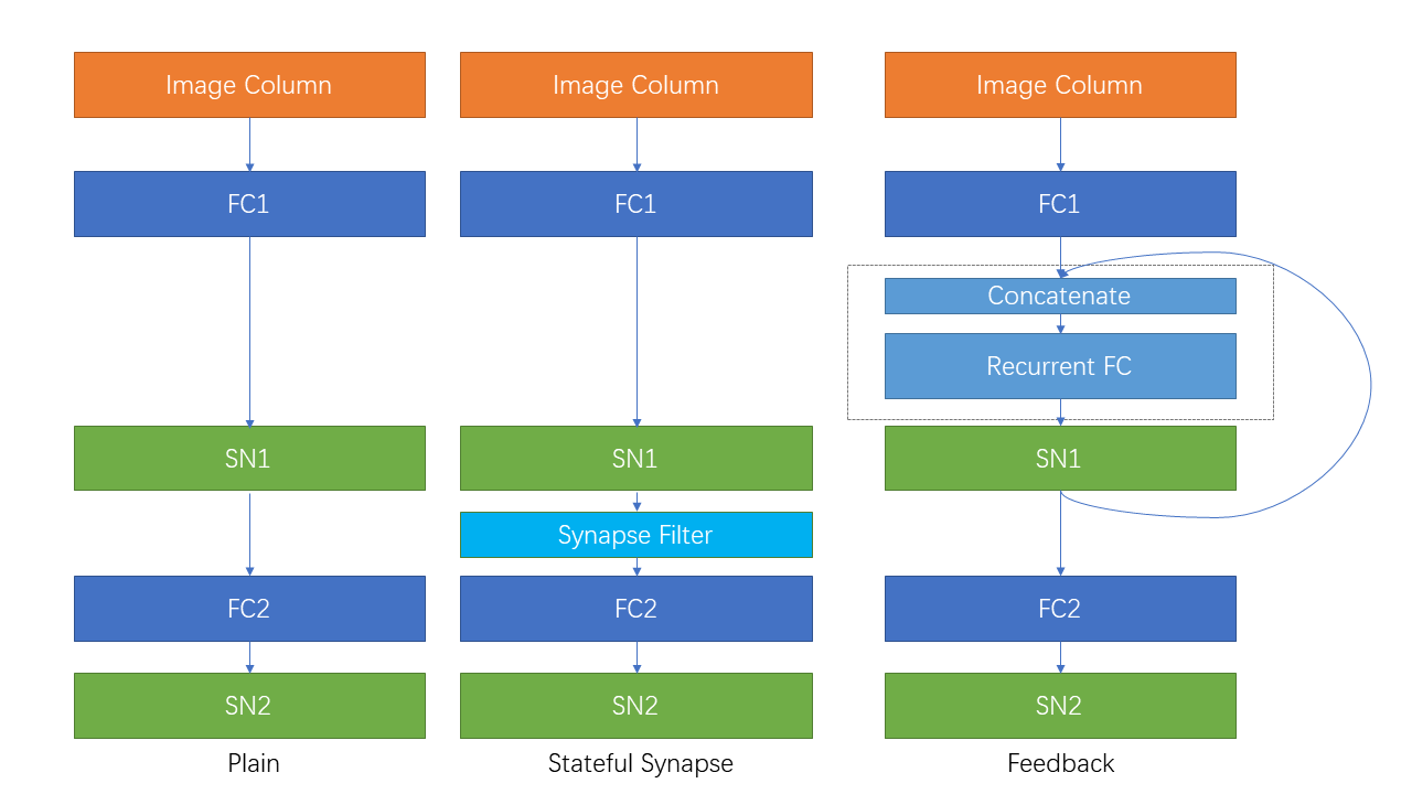
Now let us define a plain feedforward network Net:
class Net(nn.Module):
    def __init__(self):
        super().__init__()
        self.fc1 = nn.Linear(28, 32)
        self.sn1 = neuron.MultiStepIFNode(surrogate_function=surrogate.ATan(), detach_reset=True, backend=backend)
        self.fc2 = nn.Linear(32, 10)
        self.sn2 = neuron.MultiStepIFNode(surrogate_function=surrogate.ATan(), detach_reset=True, backend=backend)

    def forward(self, x: torch.Tensor):
        # x.shape = [N, C, H, W]
        x.squeeze_(1)  # [N, H, W]
        x = x.permute(2, 0, 1)  # [W, N, H]
        x = seq_to_ann_forward(x, self.fc1)
        x = self.sn1(x)
        x = seq_to_ann_forward(x, self.fc2)
        x = self.sn2(x)
        return x.mean(0)
We add spikingjelly.clock_driven.layer.SynapseFilter after the first spiking neurons layer and get StatefulSynapseNet:
class StatefulSynapseNet(nn.Module):
    def __init__(self):
        super().__init__()
        self.fc1 = nn.Linear(28, 32)
        self.sn1 = neuron.MultiStepIFNode(surrogate_function=surrogate.ATan(), detach_reset=True, backend=backend)
        self.sy1 = layer.MultiStepContainer(layer.SynapseFilter(tau=2., learnable=True))
        self.fc2 = nn.Linear(32, 10)
        self.sn2 = neuron.MultiStepIFNode(surrogate_function=surrogate.ATan(), detach_reset=True, backend=backend)

    def forward(self, x: torch.Tensor):
        # x.shape = [N, C, H, W]
        x.squeeze_(1)  # [N, H, W]
        x = x.permute(2, 0, 1)  # [W, N, H]
        x = self.fc1(x)
        x = self.sn1(x)
        x = self.sy1(x)
        x = self.fc2(x)
        x = self.sn2(x)
        return x.mean(0)
We add a recurrent connection spikingjelly.clock_driven.layer.LinearRecurrentContainer from the first spiking
neurons layer’s output to itself and get FeedBackNet:
class FeedBackNet(nn.Module):
    def __init__(self):
        super().__init__()
        self.fc1 = nn.Linear(28, 32)
        self.sn1 = layer.MultiStepContainer(
            layer.LinearRecurrentContainer(
                neuron.IFNode(surrogate_function=surrogate.ATan(), detach_reset=True),
                32, 32
            )
        )
        self.fc2 = nn.Linear(32, 10)
        self.sn2 = neuron.MultiStepIFNode(surrogate_function=surrogate.ATan(), detach_reset=True, backend=backend)

    def forward(self, x: torch.Tensor):
        # x.shape = [N, C, H, W]
        x.squeeze_(1)  # [N, H, W]
        x = x.permute(2, 0, 1)  # [W, N, H]
        x = seq_to_ann_forward(x, self.fc1)
        x = self.sn1(x)
        x = seq_to_ann_forward(x, self.fc2)
        x = self.sn2(x)
        return x.mean(0)
The following figure shows the three networks:
The complete codes are available at spikingjelly.clock_driven.examples.rsnn_sequential_fmnist. We can run it in console, and the running arguments are
(pytorch-env) PS C:/Users/fw> python -m spikingjelly.clock_driven.examples.rsnn_sequential_fmnist --h
usage: rsnn_sequential_fmnist.py [-h] [--data-path DATA_PATH] [--device DEVICE] [-b BATCH_SIZE] [--epochs N] [-j N]
                                 [--lr LR] [--opt OPT] [--lrs LRS] [--step-size STEP_SIZE] [--step-gamma STEP_GAMMA]
                                 [--cosa-tmax COSA_TMAX] [--momentum M] [--wd W] [--output-dir OUTPUT_DIR]
                                 [--resume RESUME] [--start-epoch N] [--cache-dataset] [--amp] [--tb] [--model MODEL]

PyTorch Classification Training

optional arguments:
  -h, --help            show this help message and exit
  --data-path DATA_PATH
                        dataset
  --device DEVICE       device
  -b BATCH_SIZE, --batch-size BATCH_SIZE
  --epochs N            number of total epochs to run
  -j N, --workers N     number of data loading workers (default: 16)
  --lr LR               initial learning rate
  --opt OPT             optimizer (sgd or adam)
  --lrs LRS             lr schedule (cosa(CosineAnnealingLR), step(StepLR)) or None
  --step-size STEP_SIZE
                        step_size for StepLR
  --step-gamma STEP_GAMMA
                        gamma for StepLR
  --cosa-tmax COSA_TMAX
                        T_max for CosineAnnealingLR. If none, it will be set to epochs
  --momentum M          Momentum for SGD
  --wd W, --weight-decay W
                        weight decay (default: 0)
  --output-dir OUTPUT_DIR
                        path where to save
  --resume RESUME       resume from checkpoint
  --start-epoch N       start epoch
  --cache-dataset       Cache the datasets for quicker initialization. It also serializes the transforms
  --amp                 Use AMP training
  --tb                  Use TensorBoard to record logs
  --model MODEL         "plain", "feedback", or "stateful-synapse"
Let us train the three networks:
python -m spikingjelly.clock_driven.examples.rsnn_sequential_fmnist --data-path /raid/wfang/datasets/FashionMNIST --tb --device cuda:0 --amp --model plain

python -m spikingjelly.clock_driven.examples.rsnn_sequential_fmnist --data-path /raid/wfang/datasets/FashionMNIST --tb --device cuda:1 --amp --model feedback

python -m spikingjelly.clock_driven.examples.rsnn_sequential_fmnist --data-path /raid/wfang/datasets/FashionMNIST --tb --device cuda:2 --amp --model stateful-synapse
The train loss is:

The train accuracy is:

The test accuracy is:

We can find that both feedback and stateful-synapse have higher accuracy than plain, indicating that recurrent
connections and stateful synapses can promote the network’s ability to learn long-term dependencies.
- 1
Yin B, Corradi F, Bohté S M. Effective and efficient computation with multiple-timescale spiking recurrent neural networks[C]//International Conference on Neuromorphic Systems 2020. 2020: 1-8.
- 2
Diehl P U, Cook M. Unsupervised learning of digit recognition using spike-timing-dependent plasticity[J]. Frontiers in computational neuroscience, 2015, 9: 99.
- 3
Fang H, Shrestha A, Zhao Z, et al. Exploiting Neuron and Synapse Filter Dynamics in Spatial Temporal Learning of Deep Spiking Neural Network[J].