spikingjelly.clock_driven.layer package

Module contents

class spikingjelly.clock_driven.layer.NeuNorm(in_channels, height, width, k=0.9, shared_across_channels=False)[源代码]

基类：MemoryModule

API in English

参数

in_channels – 输入数据的通道数
height – 输入数据的宽
width – 输入数据的高
k – 动量项系数
shared_across_channels – 可学习的权重 w 是否在通道这一维度上共享。设置为 True 可以大幅度节省内存

Direct Training for Spiking Neural Networks: Faster, Larger, Better 中提出的NeuNorm层。NeuNorm层必须放在二维卷积层后的脉冲神经元后，例如：

Conv2d -> LIF -> NeuNorm

要求输入的尺寸是 [batch_size, in_channels, height, width]。

in_channels 是输入到NeuNorm层的通道数，也就是论文中的 \(F\)。

k 是动量项系数，相当于论文中的 \(k_{\tau 2}\)。

论文中的 \(\frac{v}{F}\) 会根据 \(k_{\tau 2} + vF = 1\) 自动算出。

中文API

参数

in_channels – channels of input
height – height of input
width – height of width
k – momentum factor
shared_across_channels – whether the learnable parameter w is shared over channel dim. If set True, the consumption of memory can decrease largely

The NeuNorm layer is proposed in Direct Training for Spiking Neural Networks: Faster, Larger, Better.

It should be placed after spiking neurons behind convolution layer, e.g.,

Conv2d -> LIF -> NeuNorm

The input should be a 4-D tensor with shape = [batch_size, in_channels, height, width].

in_channels is the channels of input，which is \(F\) in the paper.

k is the momentum factor，which is \(k_{\tau 2}\) in the paper.

\(\frac{v}{F}\) will be calculated by \(k_{\tau 2} + vF = 1\) autonomously.

forward(in_spikes: Tensor)[源代码]

extra_repr() → str[源代码]

training: bool

class spikingjelly.clock_driven.layer.DCT(kernel_size)[源代码]

基类：Module

API in English

参数: kernel_size – 进行分块DCT变换的块大小

将输入的 shape = [*, W, H] 的数据进行分块DCT变换的层，* 表示任意额外添加的维度。变换只在最后2维进行，要求 W 和 H 都能整除 kernel_size。

DCT 是 AXAT 的一种特例。

中文API

参数: kernel_size – block size for DCT transform

Apply Discrete Cosine Transform on input with shape = [*, W, H], where * means any number of additional dimensions. DCT will only applied in the last two dimensions. W and H should be divisible by kernel_size.

Note that DCT is a special case of AXAT.

forward(x: Tensor)[源代码]

training: bool

class spikingjelly.clock_driven.layer.AXAT(in_features, out_features)[源代码]

基类：Module

API in English

参数

in_features – 输入数据的最后2维的尺寸。输入应该是 shape = [*, in_features, in_features]
out_features – 输出数据的最后2维的尺寸。输出数据为 shape = [*, out_features, out_features]

对输入数据 \(X\) 在最后2维进行线性变换 \(AXA^{T}\) 的操作，\(A\) 是 shape = [out_features, in_features] 的矩阵。

将输入的数据看作是批量个 shape = [in_features, in_features] 的矩阵.

中文API

参数

in_features – feature number of input at last two dimensions. The input should be shape = [*, in_features, in_features]
out_features – feature number of output at last two dimensions. The output will be shape = [*, out_features, out_features]

Apply \(AXA^{T}\) transform on input \(X\) at the last two dimensions. \(A\) is a tensor with shape = [out_features, in_features].

The input will be regarded as a batch of tensors with shape = [in_features, in_features].

forward(x: Tensor)[源代码]

training: bool

class spikingjelly.clock_driven.layer.Dropout(p=0.5)[源代码]

基类：MemoryModule

API in English

参数: p (float) – 每个元素被设置为0的概率

与 torch.nn.Dropout 的几乎相同。区别在于，在每一轮的仿真中，被设置成0的位置不会发生改变；直到下一轮运行，即网络调用reset()函数后，才会按照概率去重新决定，哪些位置被置0。

小技巧

这种Dropout最早由 Enabling Spike-based Backpropagation for Training Deep Neural Network Architectures 一文进行详细论述：

There is a subtle difference in the way dropout is applied in SNNs compared to ANNs. In ANNs, each epoch of training has several iterations of mini-batches. In each iteration, randomly selected units (with dropout ratio of \(p\)) are disconnected from the network while weighting by its posterior probability (\(1-p\)). However, in SNNs, each iteration has more than one forward propagation depending on the time length of the spike train. We back-propagate the output error and modify the network parameters only at the last time step. For dropout to be effective in our training method, it has to be ensured that the set of connected units within an iteration of mini-batch data is not changed, such that the neural network is constituted by the same random subset of units during each forward propagation within a single iteration. On the other hand, if the units are randomly connected at each time-step, the effect of dropout will be averaged out over the entire forward propagation time within an iteration. Then, the dropout effect would fade-out once the output error is propagated backward and the parameters are updated at the last time step. Therefore, we need to keep the set of randomly connected units for the entire time window within an iteration.

中文API

参数: p (float) – probability of an element to be zeroed

This layer is almost same with torch.nn.Dropout. The difference is that elements have been zeroed at first step during a simulation will always be zero. The indexes of zeroed elements will be update only after reset() has been called and a new simulation is started.

Tip

This kind of Dropout is firstly described in Enabling Spike-based Backpropagation for Training Deep Neural Network Architectures:

There is a subtle difference in the way dropout is applied in SNNs compared to ANNs. In ANNs, each epoch of training has several iterations of mini-batches. In each iteration, randomly selected units (with dropout ratio of \(p\)) are disconnected from the network while weighting by its posterior probability (\(1-p\)). However, in SNNs, each iteration has more than one forward propagation depending on the time length of the spike train. We back-propagate the output error and modify the network parameters only at the last time step. For dropout to be effective in our training method, it has to be ensured that the set of connected units within an iteration of mini-batch data is not changed, such that the neural network is constituted by the same random subset of units during each forward propagation within a single iteration. On the other hand, if the units are randomly connected at each time-step, the effect of dropout will be averaged out over the entire forward propagation time within an iteration. Then, the dropout effect would fade-out once the output error is propagated backward and the parameters are updated at the last time step. Therefore, we need to keep the set of randomly connected units for the entire time window within an iteration.

extra_repr()[源代码]

create_mask(x: Tensor)[源代码]

forward(x: Tensor)[源代码]

training: bool

class spikingjelly.clock_driven.layer.Dropout2d(p=0.2)[源代码]

基类：Dropout

API in English

参数: p (float) – 每个元素被设置为0的概率

与 torch.nn.Dropout2d 的几乎相同。区别在于，在每一轮的仿真中，被设置成0的位置不会发生改变；直到下一轮运行，即网络调用reset()函数后，才会按照概率去重新决定，哪些位置被置0。

关于SNN中Dropout的更多信息，参见 layer.Dropout。

中文API

参数: p (float) – probability of an element to be zeroed

This layer is almost same with torch.nn.Dropout2d. The difference is that elements have been zeroed at first step during a simulation will always be zero. The indexes of zeroed elements will be update only after reset() has been called and a new simulation is started.

For more information about Dropout in SNN, refer to layer.Dropout.

create_mask(x: Tensor)[源代码]

training: bool

class spikingjelly.clock_driven.layer.MultiStepDropout(p=0.5)[源代码]

基类：Dropout

API in English

参数: p (float) – 每个元素被设置为0的概率

spikingjelly.clock_driven.layer.Dropout 的多步版本。

小技巧

阅读传播模式以获取更多关于单步和多步传播的信息。

中文API

参数: p (float) – probability of an element to be zeroed

The multi-step version of spikingjelly.clock_driven.layer.Dropout.

Tip

Read Propagation Pattern for more details about single-step and multi-step propagation.

forward(x_seq: Tensor)[源代码]

training: bool

class spikingjelly.clock_driven.layer.MultiStepDropout2d(p=0.5)[源代码]

基类：Dropout2d

API in English

参数: p (float) – 每个元素被设置为0的概率

spikingjelly.clock_driven.layer.Dropout2d 的多步版本。

小技巧

阅读传播模式以获取更多关于单步和多步传播的信息。

中文API

参数: p (float) – probability of an element to be zeroed

The multi-step version of spikingjelly.clock_driven.layer.Dropout2d.

Tip

Read Propagation Pattern for more details about single-step and multi-step propagation.

forward(x_seq: Tensor)[源代码]

training: bool

class spikingjelly.clock_driven.layer.SynapseFilter(tau=100.0, learnable=False)[源代码]

基类：MemoryModule

API in English

参数

tau – time 突触上电流衰减的时间常数
learnable – 时间常数在训练过程中是否是可学习的。若为 True，则 tau 会被设定成时间常数的初始值

具有滤波性质的突触。突触的输出电流满足，当没有脉冲输入时，输出电流指数衰减：

\[\tau \frac{\mathrm{d} I(t)}{\mathrm{d} t} = - I(t)\]

当有新脉冲输入时，输出电流自增1：

\[I(t) = I(t) + 1\]

记输入脉冲为 \(S(t)\)，则离散化后，统一的电流更新方程为：

\[I(t) = I(t-1) - (1 - S(t)) \frac{1}{\tau} I(t-1) + S(t)\]

这种突触能将输入脉冲进行平滑，简单的示例代码和输出结果：

T = 50
in_spikes = (torch.rand(size=[T]) >= 0.95).float()
lp_syn = LowPassSynapse(tau=10.0)
pyplot.subplot(2, 1, 1)
pyplot.bar(torch.arange(0, T).tolist(), in_spikes, label='in spike')
pyplot.xlabel('t')
pyplot.ylabel('spike')
pyplot.legend()

out_i = []
for i in range(T):
    out_i.append(lp_syn(in_spikes[i]))
pyplot.subplot(2, 1, 2)
pyplot.plot(out_i, label='out i')
pyplot.xlabel('t')
pyplot.ylabel('i')
pyplot.legend()
pyplot.show()

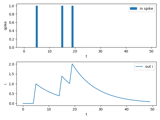
输出电流不仅取决于当前时刻的输入，还取决于之前的输入，使得该突触具有了一定的记忆能力。

这种突触偶有使用，例如：

Unsupervised learning of digit recognition using spike-timing-dependent plasticity

Exploiting Neuron and Synapse Filter Dynamics in Spatial Temporal Learning of Deep Spiking Neural Network

另一种视角是将其视为一种输入为脉冲，并输出其电压的LIF神经元。并且该神经元的发放阈值为 \(+\infty\) 。

神经元最后累计的电压值一定程度上反映了该神经元在整个仿真过程中接收脉冲的数量，从而替代了传统的直接对输出脉冲计数（即发放频率）来表示神经元活跃程度的方法。因此通常用于最后一层，在以下文章中使用：

Enabling spike-based backpropagation for training deep neural network architectures

中文API

参数

tau – time constant that determines the decay rate of current in the synapse
learnable – whether time constant is learnable during training. If True, then tau will be the initial value of time constant

The synapse filter that can filter input current. The output current will decay when there is no input spike:

\[\tau \frac{\mathrm{d} I(t)}{\mathrm{d} t} = - I(t)\]

The output current will increase 1 when there is a new input spike:

\[I(t) = I(t) + 1\]

Denote the input spike as \(S(t)\), then the discrete current update equation is as followed:

\[I(t) = I(t-1) - (1 - S(t)) \frac{1}{\tau} I(t-1) + S(t)\]

This synapse can smooth input. Here is the example and output:

T = 50
in_spikes = (torch.rand(size=[T]) >= 0.95).float()
lp_syn = LowPassSynapse(tau=10.0)
pyplot.subplot(2, 1, 1)
pyplot.bar(torch.arange(0, T).tolist(), in_spikes, label='in spike')
pyplot.xlabel('t')
pyplot.ylabel('spike')
pyplot.legend()

out_i = []
for i in range(T):
    out_i.append(lp_syn(in_spikes[i]))
pyplot.subplot(2, 1, 2)
pyplot.plot(out_i, label='out i')
pyplot.xlabel('t')
pyplot.ylabel('i')
pyplot.legend()
pyplot.show()

The output current is not only determined by the present input but also by the previous input, which makes this synapse have memory.

This synapse is sometimes used, e.g.:

Unsupervised learning of digit recognition using spike-timing-dependent plasticity

Exploiting Neuron and Synapse Filter Dynamics in Spatial Temporal Learning of Deep Spiking Neural Network

Another view is regarding this synapse as a LIF neuron with a \(+\infty\) threshold voltage.

The final output of this synapse (or the final voltage of this LIF neuron) represents the accumulation of input spikes, which substitute for traditional firing rate that indicates the excitatory level. So, it can be used in the last layer of the network, e.g.:

Enabling spike-based backpropagation for training deep neural network architectures

extra_repr()[源代码]

forward(in_spikes: Tensor)[源代码]

training: bool

class spikingjelly.clock_driven.layer.ChannelsPool(pool: MaxPool1d)[源代码]

基类：Module

API in English

参数: pool – nn.MaxPool1d 或 nn.AvgPool1d，池化层

使用 pool 将输入的4-D数据在第1个维度上进行池化。

示例代码：

>>> cp = ChannelsPool(torch.nn.MaxPool1d(2, 2))
>>> x = torch.rand(size=[2, 8, 4, 4])
>>> y = cp(x)
>>> y.shape
torch.Size([2, 4, 4, 4])

中文API

参数: pool – nn.MaxPool1d or nn.AvgPool1d, the pool layer

Use pool to pooling 4-D input at dimension 1.

Examples:

>>> cmp = ChannelsPool(torch.nn.MaxPool1d(2, 2))
>>> x = torch.rand(size=[2, 8, 4, 4])
>>> y = cp(x)
>>> y.shape
torch.Size([2, 4, 4, 4])

forward(x: Tensor)[源代码]

training: bool

class spikingjelly.clock_driven.layer.DropConnectLinear(in_features: int, out_features: int, bias: bool = True, p: float = 0.5, samples_num: int = 1024, invariant: bool = False, activation: Module = ReLU())[源代码]

基类：MemoryModule

API in English

参数

in_features (int) – 每个输入样本的特征数
out_features (int) – 每个输出样本的特征数
bias (bool) – 若为 False，则本层不会有可学习的偏置项。默认为 True
p (float) – 每个连接被断开的概率。默认为0.5
samples_num (int) – 在推理时，从高斯分布中采样的数据数量。默认为1024
invariant (bool) – 若为 True，线性层会在第一次执行前向传播时被按概率断开，断开后的线性层会保持不变，直到 reset() 函数被调用，线性层恢复为完全连接的状态。完全连接的线性层，调用 reset() 函数后的第一次前向传播时被重新按概率断开。若为 False，在每一次前向传播时线性层都会被重新完全连接再按概率断开。阅读 layer.Dropout 以获得更多关于此参数的信息。默认为 False
activation (None or nn.Module) – 在线性层后的激活层

DropConnect，由 Regularization of Neural Networks using DropConnect 一文提出。DropConnect与Dropout非常类似，区别在于DropConnect是以概率 p 断开连接，而Dropout是将输入以概率置0。

备注

在使用DropConnect进行推理时，输出的tensor中的每个元素，都是先从高斯分布中采样，通过激活层激活，再在采样数量上进行平均得到的。详细的流程可以在 Regularization of Neural Networks using DropConnect 一文中的 Algorithm 2 找到。激活层 activation 在中间的步骤起作用，因此我们将其作为模块的成员。

中文API

参数

in_features (int) – size of each input sample
out_features (int) – size of each output sample
bias (bool) – If set to False, the layer will not learn an additive bias. Default: True
p (float) – probability of an connection to be zeroed. Default: 0.5
samples_num (int) – number of samples drawn from the Gaussian during inference. Default: 1024
invariant (bool) – If set to True, the connections will be dropped at the first time of forward and the dropped connections will remain unchanged until reset() is called and the connections recovery to fully-connected status. Then the connections will be re-dropped at the first time of forward after reset(). If set to False, the connections will be re-dropped at every forward. See layer.Dropout for more information to understand this parameter. Default: False
activation (None or nn.Module) – the activation layer after the linear layer

DropConnect, which is proposed by Regularization of Neural Networks using DropConnect, is similar with Dropout but drop connections of a linear layer rather than the elements of the input tensor with probability p.

Note

When inference with DropConnect, every elements of the output tensor are sampled from a Gaussian distribution, activated by the activation layer and averaged over the sample number samples_num. See Algorithm 2 in Regularization of Neural Networks using DropConnect for more details. Note that activation is an intermediate process. This is the reason why we include activation as a member variable of this module.

reset_parameters() → None[源代码]

API in English

返回: None
返回类型: None

初始化模型中的可学习参数。

中文API

返回: None
返回类型: None

Initialize the learnable parameters of this module.

reset()[源代码]

API in English

返回: None
返回类型: None

将线性层重置为完全连接的状态，若 self.activation 也是一个有状态的层，则将其也重置。

中文API

返回: None
返回类型: None

Reset the linear layer to fully-connected status. If self.activation is also stateful, this function will also reset it.

drop(batch_size: int)[源代码]

forward(input: Tensor) → Tensor[源代码]

extra_repr() → str[源代码]

training: bool

class spikingjelly.clock_driven.layer.MultiStepContainer(*args)[源代码]

基类：Sequential

API in English

参数: args (torch.nn.Module) – 单个或多个网络模块

将单步模块包装成多步模块的包装器。

小技巧

阅读传播模式以获取更多关于单步和多步传播的信息。

中文API

参数: args (torch.nn.Module) – one or many modules

A container that wraps single-step modules to a multi-step modules.

Tip

Read Propagation Pattern for more details about single-step and multi-step propagation.

forward(x_seq: Tensor)[源代码]

参数: x_seq (Tensor) – shape=[T, batch_size, …]
返回: y_seq, shape=[T, batch_size, …]
返回类型: Tensor

training: bool

class spikingjelly.clock_driven.layer.SeqToANNContainer(*args)[源代码]

基类：Sequential

API in English

参数

*args –

无状态的单个或多个ANN网络层

包装无状态的ANN以处理序列数据的包装器。shape=[T, batch_size, ...] 的输入会被拼接成 shape=[T * batch_size, ...] 再送入被包装的模块。输出结果会被再拆成 shape=[T, batch_size, ...]。

示例代码

中文API

参数

*args –

one or many stateless ANN layers

A container that contain sataeless ANN to handle sequential data. This container will concatenate inputs shape=[T, batch_size, ...] at time dimension as shape=[T * batch_size, ...], and send the reshaped inputs to contained ANN. The output will be split to shape=[T, batch_size, ...].

Examples:

forward(x_seq: Tensor)[源代码]

参数: x_seq (Tensor) – shape=[T, batch_size, …]
返回: y_seq, shape=[T, batch_size, …]
返回类型: Tensor

training: bool

class spikingjelly.clock_driven.layer.STDPLearner(tau_pre: float, tau_post: float, f_pre, f_post)[源代码]

基类：MemoryModule

import torch
import torch.nn as nn
from spikingjelly.clock_driven import layer, neuron, functional
from matplotlib import pyplot as plt
import numpy as np
def f_pre(x):
    return x.abs() + 0.1

def f_post(x):
    return - f_pre(x)

fc = nn.Linear(1, 1, bias=False)

stdp_learner = layer.STDPLearner(100., 100., f_pre, f_post)
trace_pre = []
trace_post = []
w = []
T = 256
s_pre = torch.zeros([T, 1])
s_post = torch.zeros([T, 1])
s_pre[0: T // 2] = (torch.rand_like(s_pre[0: T // 2]) > 0.95).float()
s_post[0: T // 2] = (torch.rand_like(s_post[0: T // 2]) > 0.9).float()

s_pre[T // 2:] = (torch.rand_like(s_pre[T // 2:]) > 0.8).float()
s_post[T // 2:] = (torch.rand_like(s_post[T // 2:]) > 0.95).float()

for t in range(T):
    stdp_learner.stdp(s_pre[t], s_post[t], fc, 1e-2)
    trace_pre.append(stdp_learner.trace_pre.item())
    trace_post.append(stdp_learner.trace_post.item())
    w.append(fc.weight.item())

plt.style.use('science')
fig = plt.figure(figsize=(10, 6))
s_pre = s_pre[:, 0].numpy()
s_post = s_post[:, 0].numpy()
t = np.arange(0, T)
plt.subplot(5, 1, 1)
plt.eventplot((t * s_pre)[s_pre == 1.], lineoffsets=0, colors='r')
plt.yticks([])
plt.ylabel('$S_{pre}$', rotation=0, labelpad=10)
plt.xticks([])
plt.xlim(0, T)
plt.subplot(5, 1, 2)
plt.plot(t, trace_pre)
plt.ylabel('$tr_{pre}$', rotation=0, labelpad=10)
plt.xticks([])
plt.xlim(0, T)

plt.subplot(5, 1, 3)
plt.eventplot((t * s_post)[s_post == 1.], lineoffsets=0, colors='r')
plt.yticks([])
plt.ylabel('$S_{post}$', rotation=0, labelpad=10)
plt.xticks([])
plt.xlim(0, T)
plt.subplot(5, 1, 4)
plt.plot(t, trace_post)
plt.ylabel('$tr_{post}$', rotation=0, labelpad=10)
plt.xticks([])
plt.xlim(0, T)
plt.subplot(5, 1, 5)
plt.plot(t, w)
plt.ylabel('$w$', rotation=0, labelpad=10)
plt.xlim(0, T)

plt.show()

stdp(s_pre: Tensor, s_post: Tensor, module: Module, learning_rate: float)[源代码]

training: bool

class spikingjelly.clock_driven.layer.PrintShapeModule(ext_str='PrintShapeModule')[源代码]

基类：Module

API in English

参数: ext_str (str) – 额外打印的字符串

只打印 ext_str 和输入的 shape，不进行任何操作的网络层，可以用于debug。

中文API

参数: ext_str (str) – extra strings for printing

This layer will not do any operation but print ext_str and the shape of input, which can be used for debugging.

forward(x: Tensor)[源代码]

training: bool

class spikingjelly.clock_driven.layer.ConvBatchNorm2d(in_channels: int, out_channels: int, kernel_size: Union[int, Tuple[int, int]], stride: Union[int, Tuple[int, int]] = 1, padding: Union[int, Tuple[int, int]] = 0, dilation: Union[int, Tuple[int, int]] = 1, groups: int = 1, padding_mode: str = 'zeros', eps=1e-05, momentum=0.1, affine=True, track_running_stats=True)[源代码]

基类：Module

A fused Conv2d-BatchNorm2d module. See torch.nn.Conv2d and torch.nn.BatchNorm2d for params information.

Examples:

convbn = ConvBatchNorm2d(3, 64, kernel_size=3, padding=1)
x = torch.rand([16, 3, 224, 224])
with torch.no_grad():
    convbn.eval()
    conv = convbn.get_fused_conv()
    conv.eval()
    print((convbn(x) - conv(x)).abs().max())

    k_weight = 1.5
    b_weight = 0.4
    k_bias = 0.8
    b_bias = 0.1

    conv.weight.data *= k_weight
    conv.weight.data += b_weight
    conv.bias.data *= k_bias
    conv.bias.data += b_bias

    convbn.scale_fused_weight(k_weight, b_weight)
    convbn.scale_fused_bias(k_bias, b_bias)

    print((convbn(x) - conv(x)).abs().max())

forward(x: Tensor)[源代码]

get_fused_weight()[源代码]

返回: the weight of this fused module
返回类型: Tensor

get_fused_bias()[源代码]

返回: the bias of this fused module
返回类型: Tensor

scale_fused_weight(k=None, b=None)[源代码]

参数

k (float or None) – scale factor
b (float or None) – bias factor

Set the weight of this fused module to weight * k + b

scale_fused_bias(k=None, b=None)[源代码]

参数

k (float or None) – scale factor
b (float or None) – bias factor

Set the bias of this fused module to bias * k + b

get_fused_conv()[源代码]

training: bool

class spikingjelly.clock_driven.layer.ElementWiseRecurrentContainer(sub_module: Module, element_wise_function: Callable)[源代码]

基类：MemoryModule

参数

sub_module (torch.nn.Module) – the contained module
element_wise_function (Callable) – the user-defined element-wise function, which should have the format z=f(x, y)

A container that use a element-wise recurrent connection. Denote the inputs and outputs of sub_module as \(i[t]\) and \(y[t]\) (Note that \(y[t]\) is also the outputs of this module), and the inputs of this module as \(x[t]\), then

\[i[t] = f(x[t], y[t-1])\]

where \(f\) is the user-defined element-wise function. We set \(y[-1] = 0\).

Note

The shape inputs and outputs of sub_module must be the same.

Codes example:

T = 8
net = ElementWiseRecurrentContainer(neuron.IFNode(v_reset=None), element_wise_function=lambda x, y: x + y)
print(net)
x = torch.zeros([T])
x[0] = 1.5
for t in range(T):
    print(t, f'x[t]={x[t]}, s[t]={net(x[t])}')

functional.reset_net(net)

forward(x: Tensor)[源代码]

extra_repr() → str[源代码]

training: bool

class spikingjelly.clock_driven.layer.LinearRecurrentContainer(sub_module: Module, in_features: int, out_features: int, bias: bool = True)[源代码]

基类：MemoryModule

参数

sub_module (torch.nn.Module) – the contained module
in_features (int) – size of each input sample
out_features (int) – size of each output sample
bias (bool) – If set to False, the layer will not learn an additive bias

A container that use a linear recurrent connection. Denote the inputs and outputs of sub_module as \(i[t]\) and \(y[t]\) (Note that \(y[t]\) is also the outputs of this module), and the inputs of this module as \(x[t]\), then

\[\begin{split}i[t] = \begin{pmatrix} x[t] \\ y[t-1]\end{pmatrix} W^{T} + b\end{split}\]

where \(W, b\) are the weight and bias of the linear connection. We set \(y[-1] = 0\).

\(x[t]\) should have the shape [N, *, in_features], and \(y[t]\) has the shape [N, *, out_features].

Tip

The recurrent connection is implement by torch.nn.Linear(in_features + out_features, in_features, bias).

in_features = 4
out_features = 2
T = 8
N = 2
net = LinearRecurrentContainer(
    nn.Sequential(
        nn.Linear(in_features, out_features),
        neuron.LIFNode(),
    ),
    in_features, out_features)
print(net)
x = torch.rand([T, N, in_features])
for t in range(T):
    print(t, net(x[t]))

functional.reset_net(net)

forward(x: Tensor)[源代码]

training: bool

class spikingjelly.clock_driven.layer.MultiStepThresholdDependentBatchNorm1d(alpha: float, v_th: float, *args, **kwargs)[源代码]

基类：_MultiStepThresholdDependentBatchNormBase

API in English

参数

alpha (float) – 由网络结构决定的超参数
v_th (float) – 下一个脉冲神经元层的阈值

*args, **kwargs 中的参数与 torch.nn.BatchNorm1d 的参数相同。

Going Deeper With Directly-Trained Larger Spiking Neural Networks 一文提出的Threshold-Dependent Batch Normalization (tdBN)。

中文API

参数

alpha (float) – the hyper-parameter depending on network structure
v_th (float) – the threshold of next spiking neurons layer

Other parameters in *args, **kwargs are same with those of torch.nn.BatchNorm1d.

The Threshold-Dependent Batch Normalization (tdBN) proposed in Going Deeper With Directly-Trained Larger Spiking Neural Networks.

num_features: int

eps: float

momentum: float

affine: bool

track_running_stats: bool

class spikingjelly.clock_driven.layer.MultiStepThresholdDependentBatchNorm2d(alpha: float, v_th: float, *args, **kwargs)[源代码]

基类：_MultiStepThresholdDependentBatchNormBase

API in English

参数

alpha (float) – 由网络结构决定的超参数
v_th (float) – 下一个脉冲神经元层的阈值

*args, **kwargs 中的参数与 torch.nn.BatchNorm2d 的参数相同。

Going Deeper With Directly-Trained Larger Spiking Neural Networks 一文提出的Threshold-Dependent Batch Normalization (tdBN)。

中文API

参数

alpha (float) – the hyper-parameter depending on network structure
v_th (float) – the threshold of next spiking neurons layer

Other parameters in *args, **kwargs are same with those of torch.nn.BatchNorm2d.

The Threshold-Dependent Batch Normalization (tdBN) proposed in Going Deeper With Directly-Trained Larger Spiking Neural Networks.

num_features: int

eps: float

momentum: float

affine: bool

track_running_stats: bool

class spikingjelly.clock_driven.layer.MultiStepThresholdDependentBatchNorm3d(alpha: float, v_th: float, *args, **kwargs)[源代码]

基类：_MultiStepThresholdDependentBatchNormBase

API in English

参数

alpha (float) – 由网络结构决定的超参数
v_th (float) – 下一个脉冲神经元层的阈值

*args, **kwargs 中的参数与 torch.nn.BatchNorm3d 的参数相同。

Going Deeper With Directly-Trained Larger Spiking Neural Networks 一文提出的Threshold-Dependent Batch Normalization (tdBN)。

中文API

参数

alpha (float) – the hyper-parameter depending on network structure
v_th (float) – the threshold of next spiking neurons layer

Other parameters in *args, **kwargs are same with those of torch.nn.BatchNorm3d.

The Threshold-Dependent Batch Normalization (tdBN) proposed in Going Deeper With Directly-Trained Larger Spiking Neural Networks.

num_features: int

eps: float

momentum: float

affine: bool

track_running_stats: bool

class spikingjelly.clock_driven.layer.MultiStepTemporalWiseAttention(T: int, reduction: int = 16, dimension: int = 4)[源代码]

基类：Module

API in English

参数

T – 输入数据的时间步长
reduction – 压缩比
dimension – 输入数据的维度。当输入数据为[T, N, C, H, W]时， dimension = 4；输入数据维度为[T, N, L]时，dimension = 2。

Temporal-Wise Attention Spiking Neural Networks for Event Streams Classification 中提出的MultiStepTemporalWiseAttention层。MultiStepTemporalWiseAttention层必须放在二维卷积层之后脉冲神经元之前，例如：

Conv2d -> MultiStepTemporalWiseAttention -> LIF

输入的尺寸是 [T, N, C, H, W] 或者 [T, N, L] ，经过MultiStepTemporalWiseAttention层，输出为 [T, N, C, H, W] 或者 [T, N, L] 。

reduction 是压缩比，相当于论文中的 \(r\)。

中文API

参数

T – timewindows of input
reduction – reduction ratio
dimension – Dimensions of input. If the input dimension is [T, N, C, H, W], dimension = 4; when the input dimension is [T, N, L], dimension = 2.

The MultiStepTemporalWiseAttention layer is proposed in Temporal-Wise Attention Spiking Neural Networks for Event Streams Classification.

It should be placed after the convolution layer and before the spiking neurons, e.g.,

Conv2d -> MultiStepTemporalWiseAttention -> LIF

The dimension of the input is [T, N, C, H, W] or [T, N, L] , after the MultiStepTemporalWiseAttention layer, the output dimension is [T, N, C, H, W] or [T, N, L] .

reduction is the reduction ratio，which is \(r\) in the paper.

training: bool

forward(x_seq: Tensor)[源代码]