spikingjelly.visualizing package

Module contents

spikingjelly.visualizing.plot_2d_heatmap(array: ndarray, title: str, xlabel: str, ylabel: str, int_x_ticks=True, int_y_ticks=True, plot_colorbar=True, colorbar_y_label='magnitude', x_max=None, dpi=200)

参数

• array – shape=[T, N]的任意数组

• title – 热力图的标题

• xlabel – 热力图的x轴的label

• ylabel – 热力图的y轴的label

• int_x_ticks – x轴上是否只显示整数刻度

• int_y_ticks – y轴上是否只显示整数刻度

• plot_colorbar – 是否画出显示颜色和数值对应关系的colorbar

• colorbar_y_label – colorbar的y轴label

• x_max – 横轴的最大刻度。若设置为 None，则认为横轴的最大刻度是 array.shape[1]

• dpi – 绘图的dpi

返回

绘制好的figure

绘制一张二维的热力图。可以用来绘制一张表示多个神经元在不同时刻的电压的热力图，示例代码：

import torch
from spikingjelly.clock_driven import neuron
from spikingjelly import visualizing
from matplotlib import pyplot as plt
import numpy as np

lif = neuron.LIFNode(tau=100.)
x = torch.rand(size=[32]) * 4
T = 50
s_list = []
v_list = []
for t in range(T):
    s_list.append(lif(x).unsqueeze(0))
    v_list.append(lif.v.unsqueeze(0))

s_list = torch.cat(s_list)
v_list = torch.cat(v_list)

visualizing.plot_2d_heatmap(array=np.asarray(v_list), title='Membrane Potentials', xlabel='Simulating Step',
                            ylabel='Neuron Index', int_x_ticks=True, x_max=T, dpi=200)
plt.show()

spikingjelly.visualizing.plot_2d_bar_in_3d(array: ndarray, title: str, xlabel: str, ylabel: str, zlabel: str, int_x_ticks=True, int_y_ticks=True, int_z_ticks=False, dpi=200)

参数

• array – shape=[T, N]的任意数组

• title – 图的标题

• xlabel – x轴的label

• ylabel – y轴的label

• zlabel – z轴的label

• int_x_ticks – x轴上是否只显示整数刻度

• int_y_ticks – y轴上是否只显示整数刻度

• int_z_ticks – z轴上是否只显示整数刻度

• dpi – 绘图的dpi

返回

绘制好的figure

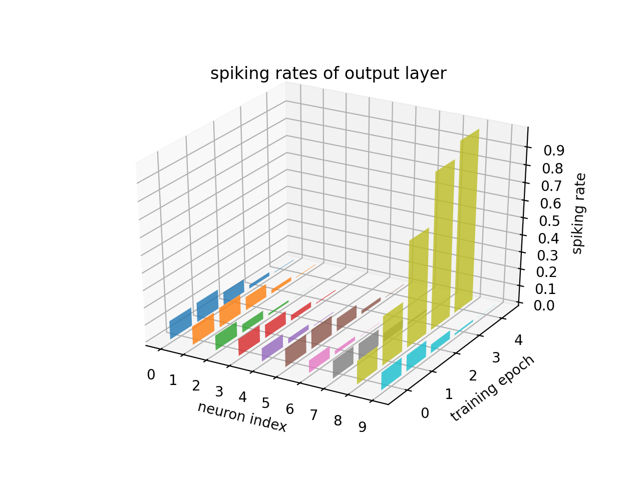
将shape=[T, N]的任意数组，绘制为三维的柱状图。可以用来绘制多个神经元的脉冲发放频率，随着时间的变化情况，示例代码：

import torch
from spikingjelly import visualizing
from matplotlib import pyplot as plt

Epochs = 5
N = 10
firing_rate = torch.zeros(Epochs, N)
init_firing_rate = torch.rand(size=[N])
for i in range(Epochs):
    firing_rate[i] = torch.softmax(init_firing_rate * (i + 1) ** 2, dim=0)
visualizing.plot_2d_bar_in_3d(firing_rate.numpy(), title='spiking rates of output layer', xlabel='neuron index',
                              ylabel='training epoch', zlabel='spiking rate', int_x_ticks=True, int_y_ticks=True,
                              int_z_ticks=False, dpi=200)
plt.show()

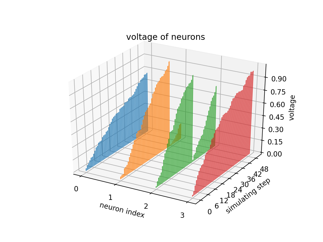
也可以用来绘制一张表示多个神经元在不同时刻的电压的热力图，示例代码：

import torch
from spikingjelly import visualizing
from matplotlib import pyplot as plt
from spikingjelly.clock_driven import neuron

neuron_num = 4
T = 50
lif_node = neuron.LIFNode(tau=100.)
w = torch.rand([neuron_num]) * 10
v_list = []
for t in range(T):
    lif_node(w * torch.rand(size=[neuron_num]))
    v_list.append(lif_node.v.unsqueeze(0))

v_list = torch.cat(v_list)
visualizing.plot_2d_bar_in_3d(v_list, title='voltage of neurons', xlabel='neuron index',
                              ylabel='simulating step', zlabel='voltage', int_x_ticks=True, int_y_ticks=True,
                              int_z_ticks=False, dpi=200)
plt.show()

spikingjelly.visualizing.plot_1d_spikes(spikes: asarray, title: str, xlabel: str, ylabel: str, int_x_ticks=True, int_y_ticks=True, plot_firing_rate=True, firing_rate_map_title='Firing Rate', dpi=200)

参数

• spikes – shape=[T, N]的np数组，其中的元素只为0或1，表示N个时长为T的脉冲数据

• title – 热力图的标题

• xlabel – 热力图的x轴的label

• ylabel – 热力图的y轴的label

• int_x_ticks – x轴上是否只显示整数刻度

• int_y_ticks – y轴上是否只显示整数刻度

• plot_firing_rate – 是否画出各个脉冲发放频率

• firing_rate_map_title – 脉冲频率发放图的标题

• dpi – 绘图的dpi

返回

绘制好的figure

画出N个时长为T的脉冲数据。可以用来画N个神经元在T个时刻的脉冲发放情况，示例代码：

import torch
from spikingjelly.clock_driven import neuron
from spikingjelly import visualizing
from matplotlib import pyplot as plt
import numpy as np

lif = neuron.LIFNode(tau=100.)
x = torch.rand(size=[32]) * 4
T = 50
s_list = []
v_list = []
for t in range(T):
    s_list.append(lif(x).unsqueeze(0))
    v_list.append(lif.v.unsqueeze(0))

s_list = torch.cat(s_list)
v_list = torch.cat(v_list)

visualizing.plot_1d_spikes(spikes=np.asarray(s_list), title='Membrane Potentials', xlabel='Simulating Step',
                           ylabel='Neuron Index', dpi=200)
plt.show()

spikingjelly.visualizing.plot_2d_spiking_feature_map(spikes: asarray, nrows, ncols, space, title: str, dpi=200)

参数

• spikes – shape=[C, W, H]，C个尺寸为W * H的脉冲矩阵，矩阵中的元素为0或1。这样的矩阵一般来源于卷积层后的脉冲神经元的输出

• nrows – 画成多少行

• ncols – 画成多少列

• space – 矩阵之间的间隙

• title – 图的标题

• dpi – 绘图的dpi

返回

一个figure，将C个矩阵全部画出，然后排列成nrows行ncols列

将C个尺寸为W * H的脉冲矩阵，全部画出，然后排列成nrows行ncols列。这样的矩阵一般来源于卷积层后的脉冲神经元的输出，通过这个函数可以对输出进行可视化。示例代码：

from spikingjelly import visualizing
import numpy as np
from matplotlib import pyplot as plt

C = 48
W = 8
H = 8
spikes = (np.random.rand(C, W, H) > 0.8).astype(float)
visualizing.plot_2d_spiking_feature_map(spikes=spikes, nrows=6, ncols=8, space=2, title='Spiking Feature Maps', dpi=200)
plt.show()

spikingjelly.visualizing.plot_one_neuron_v_s(v: ndarray, s: ndarray, v_threshold=1.0, v_reset=0.0, title='$V_{t}$ and $S_{t}$ of the neuron', dpi=200)

参数

• v – shape=[T], 存放神经元不同时刻的电压

• s – shape=[T], 存放神经元不同时刻释放的脉冲

• v_threshold – 神经元的阈值电压

• v_reset – 神经元的重置电压。也可以为 None

• title – 图的标题

• dpi – 绘图的dpi

返回

一个figure

绘制单个神经元的电压、脉冲随着时间的变化情况。示例代码：

import torch
from spikingjelly.clock_driven import neuron
from spikingjelly import visualizing
from matplotlib import pyplot as plt

lif = neuron.LIFNode(tau=100.)
x = torch.Tensor([2.0])
T = 150
s_list = []
v_list = []
for t in range(T):
    s_list.append(lif(x))
    v_list.append(lif.v)
visualizing.plot_one_neuron_v_s(v_list, s_list, v_threshold=lif.v_threshold, v_reset=lif.v_reset,
                                dpi=200)
plt.show()