STDP Learning

Author: fangwei123456

Researchers of SNNs are always interested in biological learning rules. In SpkingJelly, STDP(Spike Timing Dependent Plasticity) is also provided and can be applied to convolutional or linear layers.

STDP(Spike Timing Dependent Plasticity)

STDP(Spike Timing Dependent Plasticity) is proposed by [1], which is a synaptic plasticity rule found in biological neural system. The experiments in the biological neural systems find that the weight of synapse is influenced by the firing time of spikes of the pre and post neuron. More specific, STDP can be formulated as:

If the pre neuron fires early and the post neuron fires later, then the weight will increase; If the pre neuron fires later while the post neuron fires early, then the weight will decrease.

The curve [2] that fits the experiments data is as follows:

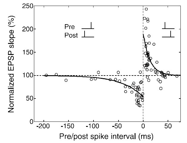
We can use the following equation to describe STDP:

\[\begin{split}\begin{align} \begin{split} \Delta w_{ij} = \begin{cases} A\exp(\frac{-|t_{i}-t_{j}|}{\tau_{+}}) , t_{i} \leq t_{j}, A > 0\\ B\exp(\frac{-|t_{i}-t_{j}|}{\tau_{-}}) , t_{i} > t_{j}, B < 0 \end{cases} \end{split} \end{align}\end{split}\]

where \(A, B\) are the maximum of weight variation, and \(\tau_{+}, \tau_{-}\) are time constants.

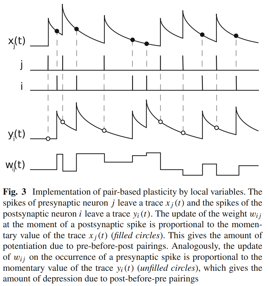
However, the above equation is seldom used in practicals because it needs to record all firing times of pre and post neurons.The trace method [3] is a more popular method to implement STDP.

For the pre neuron \(i\) and the post neuron \(j\), we use the traces \(tr_{pre}[i]\) and \(tr_{post}[j]\) to track their firing. The update of traces are similar to the LIF neuron:

\[ \begin{align}\begin{aligned}tr_{pre}[i][t] = tr_{pre}[i][t] -\frac{tr_{pre}[i][t-1]}{\tau_{pre}} + s[i][t]\\tr_{post}[j][t] = tr_{pre}[i][t] -\frac{tr_{post}[j][t-1]}{\tau_{post}} + s[j][t]\end{aligned}\end{align} \]

where \(\tau_{pre}, \tau_{post}\) are time constants of the pre and post neuron. \(s[i][t], s[j][t]\) are the spikes at time-step \(t\) of the pre neuron \(i\) and the post neuron \(j\), which can only be 0 or 1.

The update of weight is:

\[\Delta W[i][j][t] = F_{post}(w[i][j][t]) \cdot tr_{i}[t] \cdot s[j][t] - F_{pre}(w[i][j][t]) \cdot tr_{j}[t] \cdot s[i][t]\]

where \(F_{pre}, F_{post}\) are functions that control how weight changes.

STDP Learner

spikingjelly.activation_based.learning.STDPLearner can apply STDP learning on convolutional or linear layers. Please read the api doc first to learn how to use it.

Now let us use STDPLearner to build the simplest 1x1 SNN with only one pre and one post neuron. And we set the weight as 0.4:

import torch
import torch.nn as nn
from spikingjelly.activation_based import neuron, layer, learning
from matplotlib import pyplot as plt
torch.manual_seed(0)

def f_weight(x):
    return torch.clamp(x, -1, 1.)

tau_pre = 2.
tau_post = 2.
T = 128
N = 1
lr = 0.01
net = nn.Sequential(
    layer.Linear(1, 1, bias=False),
    neuron.IFNode()
)
nn.init.constant_(net[0].weight.data, 0.4)

STDPLearner can add the negative weight variation - delta_w * scale on the gradient of weight, which makes it compatible with deep learning methods. We can use the optimizer, learning rate scheduler with STDPLearner together.

In this example, we use the simplest parameter update method:

\[W = W - lr \cdot \nabla W\]

where \(\nabla W\) is - delta_w * scale. Thus, the optimizer will apply weight.data = weight.data - lr * weight.grad = weight.data + lr * delta_w * scale.

We can implement the above parameter update method by the plain torch.optim.SGD with momentum=0.:

optimizer = torch.optim.SGD(net.parameters(), lr=lr, momentum=0.)

Then we create the input spikes and set STDPLearner:

in_spike = (torch.rand([T, N, 1]) > 0.7).float()
stdp_learner = learning.STDPLearner(step_mode='s', synapse=net[0], sn=net[1], tau_pre=tau_pre, tau_post=tau_post,
                                    f_pre=f_weight, f_post=f_weight)

Then we send data to the network. Note that to plot the figure, we will squeeze() the data, which reshape them from shape = [T, N, 1] to shape = [T]:

out_spike = []
trace_pre = []
trace_post = []
weight = []
with torch.no_grad():
    for t in range(T):
        optimizer.zero_grad()
        out_spike.append(net(in_spike[t]).squeeze())
        stdp_learner.step(on_grad=True)  # add ``- delta_w * scale`` on grad
        optimizer.step()
        weight.append(net[0].weight.data.clone().squeeze())
        trace_pre.append(stdp_learner.trace_pre.squeeze())
        trace_post.append(stdp_learner.trace_post.squeeze())

in_spike = in_spike.squeeze()
out_spike = torch.stack(out_spike)
trace_pre = torch.stack(trace_pre)
trace_post = torch.stack(trace_post)
weight = torch.stack(weight)

The complete codes are available at spikingjelly/activation_based/examples/stdp_trace.py:

Let us plot in_spike, out_spike, trace_pre, trace_post, weight:

This figure is similar to Fig.3 in [3] (note that they use j as the pre neuron and i as the post neuron, while we use the opposite symbol):

Combine STDP Learning with Gradient Descent

A widely used method with STDP is using gradient descent and STDP to train different layers in an SNN. With STDPLearner, we can combine STDP learning with gradient descent easily.

Our goal is to build a deep SNN, train convolutional layers with STDP, and train linear layers with gradient descent. First, let us define the hyper-parameters:

import torch
import torch.nn as nn
import torch.nn.functional as F
from torch.optim import SGD, Adam
from spikingjelly.activation_based import learning, layer, neuron, functional

T = 8
N = 2
C = 3
H = 32
W = 32
lr = 0.1
tau_pre = 2.
tau_post = 100.
step_mode = 'm'

Here we use the input with shape = [T, N, C, H, W] = [8, 2, 3, 32, 32].

Then we define the weight function and the SNN. Here we build a convolutional SNN with a multi-step mode:

def f_weight(x):
    return torch.clamp(x, -1, 1.)


net = nn.Sequential(
    layer.Conv2d(3, 16, kernel_size=3, stride=1, padding=1, bias=False),
    neuron.IFNode(),
    layer.MaxPool2d(2, 2),
    layer.Conv2d(16, 16, kernel_size=3, stride=1, padding=1, bias=False),
    neuron.IFNode(),
    layer.MaxPool2d(2, 2),
    layer.Flatten(),
    layer.Linear(16 * 8 * 8, 64, bias=False),
    neuron.IFNode(),
    layer.Linear(64, 10, bias=False),
    neuron.IFNode(),
)

functional.set_step_mode(net, step_mode)

We want to use STDP to train layer.Conv2d while other layers are to be trained with gradient descent. We use instances_stdp as the layers which are trained by STDP:

instances_stdp = (layer.Conv2d, )

We create an STDP learner for each layer in the SNN with the instance in instances_stdp:

stdp_learners = []

for i in range(net.__len__()):
    if isinstance(net[i], instances_stdp):
        stdp_learners.append(
            learning.STDPLearner(step_mode=step_mode, synapse=net[i], sn=net[i+1], tau_pre=tau_pre, tau_post=tau_post,
                                f_pre=f_weight, f_post=f_weight)
        )

Now we split parameters into two groups. The parameters from layers whose instances are in or not in instances_stdp will be set to two optimizers. Here we use Adam to optimize the parameters which are trained by gradient descent, and SGD to optimize the parameters which are trained by STDP:

params_stdp = []
for m in net.modules():
    if isinstance(m, instances_stdp):
        for p in m.parameters():
            params_stdp.append(p)

params_stdp_set = set(params_stdp)
params_gradient_descent = []
for p in net.parameters():
    if p not in params_stdp_set:
        params_gradient_descent.append(p)

optimizer_gd = Adam(params_gradient_descent, lr=lr)
optimizer_stdp = SGD(params_stdp, lr=lr, momentum=0.)

When we train the SNN in actual tasks, e.g., classifying CIFAR-10, we get samples from the dataset. But here we only want to implement an example. Hence, we create the samples manually:

x_seq = (torch.rand([T, N, C, H, W]) > 0.5).float()
target = torch.randint(low=0, high=10, size=[N])

Then we will use the two optimizers to update the parameters. Note that the following codes are different from the plain gradient descent we use before.

First, let us clear all gradients, do a forward, calculate the loss and do a backward:

optimizer_gd.zero_grad()
optimizer_stdp.zero_grad()
y = net(x_seq).mean(0)
loss = F.cross_entropy(y, target)
loss.backward()

Note that even though optimizer_gd will only update parameters in params_gradient_descent, loss.backward() will calculate and set .grad to all parameters including those we want to calculate the weight variation (implemented by on .grad) by STDP.

Thus, we need to clear the gradients of params_stdp:

optimizer_stdp.zero_grad()

Then we need to use STDPLearner to get “gradients”, and use two optimizers to update all parameters:

for i in range(stdp_learners.__len__()):
    stdp_learners[i].step(on_grad=True)

optimizer_gd.step()
optimizer_stdp.step()

All the learners ( STDPLearner , for instance) inherit from MemoryModule. Hence, they have internal memories ( trace_pre, trace_post for STDPLearner ). In addition, the monitors inside the learners record the firing histories of the pre-synaptic and post-synaptic neurons; these histories may also be considered as internal memories of the learners. We should call the reset() method to clear the internal memory promptly so as to avoid the nonstop growing of memory consumption. We suggest resetting the learners together with the network after each batch:

functional.reset_net(net)
for i in range(stdp_learners.__len__()):
    stdp_learners[i].reset()

The complete codes are as follows:

import torch
import torch.nn as nn
import torch.nn.functional as F
from torch.optim import SGD, Adam
from spikingjelly.activation_based import learning, layer, neuron, functional

T = 8
N = 2
C = 3
H = 32
W = 32
lr = 0.1
tau_pre = 2.
tau_post = 100.
step_mode = 'm'

def f_weight(x):
    return torch.clamp(x, -1, 1.)


net = nn.Sequential(
    layer.Conv2d(3, 16, kernel_size=3, stride=1, padding=1, bias=False),
    neuron.IFNode(),
    layer.MaxPool2d(2, 2),
    layer.Conv2d(16, 16, kernel_size=3, stride=1, padding=1, bias=False),
    neuron.IFNode(),
    layer.MaxPool2d(2, 2),
    layer.Flatten(),
    layer.Linear(16 * 8 * 8, 64, bias=False),
    neuron.IFNode(),
    layer.Linear(64, 10, bias=False),
    neuron.IFNode(),
)

functional.set_step_mode(net, step_mode)

instances_stdp = (layer.Conv2d, )

stdp_learners = []

for i in range(net.__len__()):
    if isinstance(net[i], instances_stdp):
        stdp_learners.append(
            learning.STDPLearner(step_mode=step_mode, synapse=net[i], sn=net[i+1], tau_pre=tau_pre, tau_post=tau_post,
                                f_pre=f_weight, f_post=f_weight)
        )


params_stdp = []
for m in net.modules():
    if isinstance(m, instances_stdp):
        for p in m.parameters():
            params_stdp.append(p)

params_stdp_set = set(params_stdp)
params_gradient_descent = []
for p in net.parameters():
    if p not in params_stdp_set:
        params_gradient_descent.append(p)

optimizer_gd = Adam(params_gradient_descent, lr=lr)
optimizer_stdp = SGD(params_stdp, lr=lr, momentum=0.)



x_seq = (torch.rand([T, N, C, H, W]) > 0.5).float()
target = torch.randint(low=0, high=10, size=[N])

optimizer_gd.zero_grad()
optimizer_stdp.zero_grad()

y = net(x_seq).mean(0)
loss = F.cross_entropy(y, target)
loss.backward()



optimizer_stdp.zero_grad()

for i in range(stdp_learners.__len__()):
    stdp_learners[i].step(on_grad=True)

optimizer_gd.step()
optimizer_stdp.step()

functional.reset_net(net)
for i in range(stdp_learners.__len__()):
    stdp_learners[i].reset()

[1]

Bi, Guo-qiang, and Mu-ming Poo. “Synaptic modifications in cultured hippocampal neurons: dependence on spike timing, synaptic strength, and postsynaptic cell type.” Journal of neuroscience 18.24 (1998): 10464-10472.

[2]

Froemke, Robert C., et al. “Contribution of individual spikes in burst-induced long-term synaptic modification.” Journal of neurophysiology (2006).

[3] (1,2)

Morrison, Abigail, Markus Diesmann, and Wulfram Gerstner. “Phenomenological models of synaptic plasticity based on spike timing.” Biological cybernetics 98.6 (2008): 459-478.