Recurrent Connection and Stateful Synapse
Author: fangwei123456
Self-connected Modules
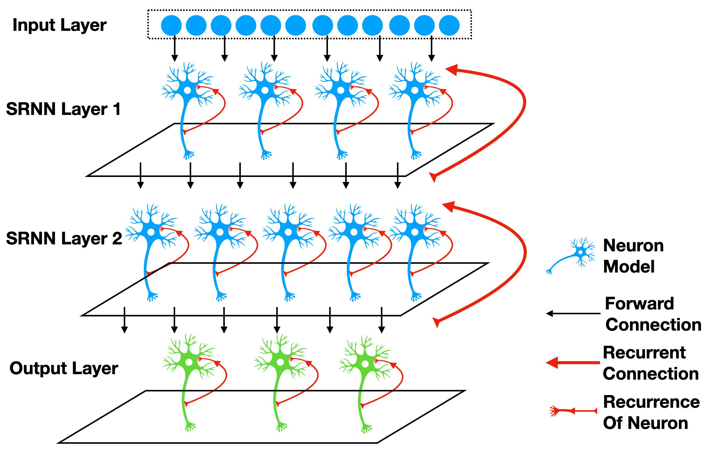
Recurrent connection is the connection from outputs to inputs, e.g., the SRNN(recurrent networks of spiking neurons) in [1], which are shown in the following figure:

We can add recurrent connection to modules by SpikingJelly easily. Considering the most simple case that we add a recurrent connection to the spiking neruons layer to make its outputs \(s[t]\) at time-step \(t\) add to the external input \(x[t+1]\) as the input to the neuron at the next time-step. We can use spikingjelly.activation_based.layer.ElementWiseRecurrentContainer to implement this idea.ElementWiseRecurrentContainer is a container that add a recurrent connection to any sub_module.The connection can be specified as a user-defined element-wise operation \(z=f(x, y)\). Denote \(x[t]\) as the external input for the whole module (container and sub_module) at time-step \(t\), \(i[t]\) and \(y[t]\) are the input and output of sub_module (note that \(y[t]\) is also the outputs of the whole module), then we can get
where \(f\) is a user-defined element-wise function. We regard \(y[-1] = 0\).
Let us use ElementWiseRecurrentContainer to wrap one IF neuron. We set the element-wise function as addition:
The external intpus are \(x[t]=[1.5, 0, ..., 0]\):
import torch
from spikingjelly.activation_based import layer, functional, neuron

T = 8
N = 1

def element_wise_add(x, y):
    return x + y

net = layer.ElementWiseRecurrentContainer(neuron.IFNode(), element_wise_add)
print(net)
x = torch.zeros([T, N])
x[0] = 1.5
for t in range(T):
    print(t, f'x[t]={x[t]}, s[t]={net(x[t])}')

functional.reset_net(net)
The outputs are:
ElementWiseRecurrentContainer(
element-wise function=<function element_wise_add at 0x00000158FC15ACA0>, step_mode=s
(sub_module): IFNode(
    v_threshold=1.0, v_reset=0.0, detach_reset=False, step_mode=s, backend=torch
    (surrogate_function): Sigmoid(alpha=4.0, spiking=True)
)
)
0 x[t]=tensor([1.5000]), s[t]=tensor([1.])
1 x[t]=tensor([0.]), s[t]=tensor([1.])
2 x[t]=tensor([0.]), s[t]=tensor([1.])
3 x[t]=tensor([0.]), s[t]=tensor([1.])
4 x[t]=tensor([0.]), s[t]=tensor([1.])
5 x[t]=tensor([0.]), s[t]=tensor([1.])
6 x[t]=tensor([0.]), s[t]=tensor([1.])
7 x[t]=tensor([0.]), s[t]=tensor([1.])
We can find that even when \(t \ge 1\), \(x[t]=0\), the neuron can still fire spikes because of the recurrent connection.
We can use spikingjelly.activation_based.layer.LinearRecurrentContainer to implement the more complex recurrent connection.
Stateful Synapse
Some papers, e.g., [2] and [3] , use the stateful synapses. By placing spikingjelly.activation_based.layer.SynapseFilter after the synapse to filter the output current, we can get the stateful synapse:
import torch
import torch.nn as nn
from spikingjelly.activation_based import layer, functional, neuron

stateful_conv = nn.Sequential(
    layer.Conv2d(3, 16, kernel_size=3, padding=1, stride=1),
    layer.SynapseFilter(tau=100.)
)
Experiments on Sequential FashionMNIST
Now let us do some simple experiments on Sequential FashionMNIST to verify whether the recurrent connection or the stateful synapse can promote the network’s ability on the memory task. The Sequential FashionMNIST dataset is a modified FashionMNIST dataset. Images will be sent to the network row by row or column by column, rather than be sent entirely. To classify correctly, the network should have good memory ability. We will send images column by column, which is similar to how humans read the book from left to right:

The following figure shows the column that is being sent:

First, let us import some packages:
import torch
import torch.nn as nn
import torch.nn.functional as F
import torchvision.datasets
from spikingjelly.activation_based import neuron, surrogate, layer, functional
from torch.cuda import amp
import os, argparse
from torch.utils.tensorboard import SummaryWriter
import time
import datetime
import sys
Define the plain feedforward network PlainNet:
class PlainNet(nn.Module):
    def __init__(self):
        super().__init__()
        self.fc = nn.Sequential(
            layer.Linear(28, 32),
            neuron.IFNode(surrogate_function=surrogate.ATan()),
            layer.Linear(32, 10),
            neuron.IFNode(surrogate_function=surrogate.ATan())
        )

    def forward(self, x: torch.Tensor):
        return self.fc(x).mean(0)
By adding a spikingjelly.activation_based.layer.SynapseFilter behind the first spiking neurons layer of PlainNet, we can get the network StatefulSynapseNet:
class StatefulSynapseNet(nn.Module):
    def __init__(self):
        super().__init__()
        self.fc = nn.Sequential(
            layer.Linear(28, 32),
            neuron.IFNode(surrogate_function=surrogate.ATan()),
            layer.SynapseFilter(tau=2., learnable=True),
            layer.Linear(32, 10),
            neuron.IFNode(surrogate_function=surrogate.ATan())
        )

    def forward(self, x: torch.Tensor):
        return self.fc(x).mean(0)
By adding a recurrent connection implemented by spikingjelly.activation_based.layer.LinearRecurrentContainer to PlainNet, we can get FeedBackNet
class FeedBackNet(nn.Module):
    def __init__(self):
        super().__init__()

        self.fc = nn.Sequential(
            layer.Linear(28, 32),
            layer.LinearRecurrentContainer(
                neuron.IFNode(surrogate_function=surrogate.ATan(), detach_reset=True),
                in_features=32, out_features=32, bias=True
            ),
            layer.Linear(32, 10),
            neuron.IFNode(surrogate_function=surrogate.ATan())
        )

    def forward(self, x: torch.Tensor):
        return self.fc(x).mean(0)
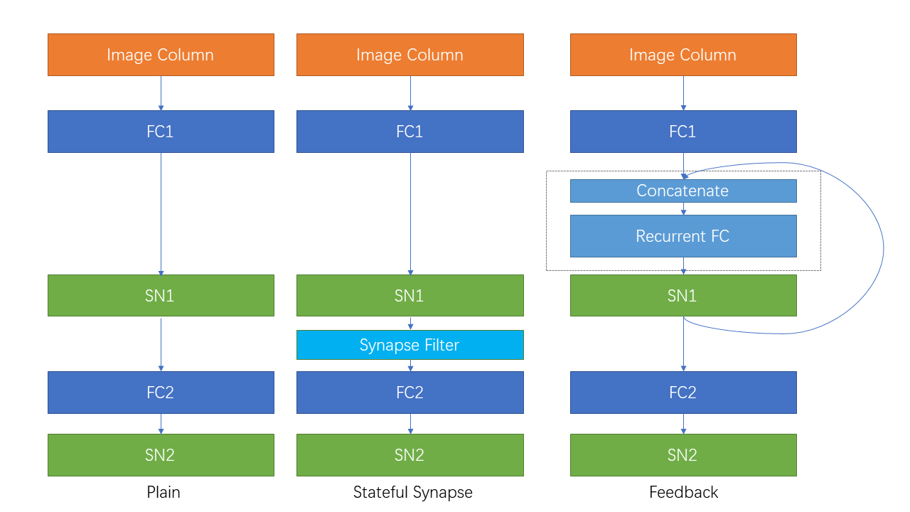
The following figure shows the network structure of three networks:

The complete codes are saved in spikingjelly.activation_based.examples.rsnn_sequential_fmnist. We can run by the following commands:
usage: rsnn_sequential_fmnist.py [-h] [-model MODEL] [-device DEVICE] [-b B] [-epochs N] [-j N] [-data-dir DATA_DIR] [-out-dir OUT_DIR] [-resume RESUME] [-amp] [-cupy] [-opt OPT] [-momentum MOMENTUM] [-lr LR]

Classify Sequential Fashion-MNIST

optional arguments:
-h, --help          show this help message and exit
-model MODEL        use which model, "plain", "ss" (StatefulSynapseNet) or "fb" (FeedBackNet)
-device DEVICE      device
-b B                batch size
-epochs N           number of total epochs to run
-j N                number of data loading workers (default: 4)
-data-dir DATA_DIR  root dir of Fashion-MNIST dataset
-out-dir OUT_DIR    root dir for saving logs and checkpoint
-resume RESUME      resume from the checkpoint path
-amp                automatic mixed precision training
-cupy               use cupy backend
-opt OPT            use which optimizer. SDG or Adam
-momentum MOMENTUM  momentum for SGD
-lr LR              learning rate
Train three networks:
python -m spikingjelly.activation_based.examples.rsnn_sequential_fmnist -device cuda:0 -b 256 -epochs 64 -data-dir /datasets/FashionMNIST/ -amp -cupy -opt sgd -lr 0.1 -j 8 -model plain

python -m spikingjelly.activation_based.examples.rsnn_sequential_fmnist -device cuda:0 -b 256 -epochs 64 -data-dir /datasets/FashionMNIST/ -amp -cupy -opt sgd -lr 0.1 -j 8 -model fb

python -m spikingjelly.activation_based.examples.rsnn_sequential_fmnist -device cuda:0 -b 256 -epochs 64 -data-dir /datasets/FashionMNIST/ -amp -cupy -opt sgd -lr 0.1 -j 8 -model ss
The following figures show the accuracy curves during training:
We can find that both StatefulSynapseNet and FeedBackNet have higher accuracy than PlainNet, indicating that recurrent connection and stateful synapse can promote the network’s memory ability.