ANN转换SNN
本教程作者: DingJianhao, fangwei123456, Lv Liuzhenghao
本节教程主要关注 spikingjelly.activation_based.ann2snn,介绍如何将训练好的ANN转换SNN,并且在SpikingJelly框架上进行仿真。
相关API见此处 API参考 。
较早的实现方案中有两套实现:基于ONNX 和 基于PyTorch。本版本基于torch.fx。fx专门用于对nn.Module实例进行转换,而且在构建计算图时会原生地将复杂模型解耦合。一起来看看吧!
ANN转换SNN的理论基础
SNN相比于ANN,产生的脉冲是离散的,这有利于高效的通信。在ANN大行其道的今天,SNN的直接训练需要较多资源。自然我们会想到使用现在非常成熟的ANN转换到SNN,希望SNN也能有类似的表现。这就牵扯到如何搭建起ANN和SNN桥梁的问题。现在SNN主流的方式是采用频率编码,因此对于输出层,我们会用神经元输出脉冲数来判断类别。发放率和ANN有没有关系呢?
幸运的是,ANN中的ReLU神经元非线性激活和SNN中IF神经元(采用减去阈值 \(V_{threshold}\) 方式重置)的发放率有着极强的相关性,我们可以借助这个特性来进行转换。这里说的神经元更新方式,也就是 神经元教程 中提到的Soft方式。
实验:IF神经元脉冲发放频率和输入的关系
我们给与恒定输入到IF神经元,观察其输出脉冲和脉冲发放频率。首先导入相关的模块,新建IF神经元层,确定输入并画出每个IF神经元的输入 \(x_{i}\):
import torch
from spikingjelly.activation_based import neuron
from spikingjelly import visualizing
from matplotlib import pyplot as plt
import numpy as np

plt.rcParams['figure.dpi'] = 200
if_node = neuron.IFNode(v_reset=None)
T = 128
x = torch.arange(-0.2, 1.2, 0.04)
plt.scatter(torch.arange(x.shape[0]), x)
plt.title('Input $x_{i}$ to IF neurons')
plt.xlabel('Neuron index $i$')
plt.ylabel('Input $x_{i}$')
plt.grid(linestyle='-.')
plt.show()

接下来,将输入送入到IF神经元层,并运行 T=128 步,观察各个神经元发放的脉冲、脉冲发放频率:
s_list = []
for t in range(T):
    s_list.append(if_node(x).unsqueeze(0))

out_spikes = np.asarray(torch.cat(s_list))
visualizing.plot_1d_spikes(out_spikes, 'IF neurons\' spikes and firing rates', 't', 'Neuron index $i$')
plt.show()

可以发现,脉冲发放的频率在一定范围内,与输入 \(x_{i}\) 的大小成正比。
接下来,让我们画出IF神经元脉冲发放频率和输入 \(x_{i}\) 的曲线,并与 \(\mathrm{ReLU}(x_{i})\) 对比:
plt.subplot(1, 2, 1)
firing_rate = np.mean(out_spikes, axis=1)
plt.plot(x, firing_rate)
plt.title('Input $x_{i}$ and firing rate')
plt.xlabel('Input $x_{i}$')
plt.ylabel('Firing rate')
plt.grid(linestyle='-.')

plt.subplot(1, 2, 2)
plt.plot(x, x.relu())
plt.title('Input $x_{i}$ and ReLU($x_{i}$)')
plt.xlabel('Input $x_{i}$')
plt.ylabel('ReLU($x_{i}$)')
plt.grid(linestyle='-.')
plt.show()

可以发现,两者的曲线几乎一致。需要注意的是,脉冲频率不可能高于1,因此IF神经元无法拟合ANN中ReLU的输入大于1的情况。
理论证明
文献 1 对ANN转SNN提供了解析的理论基础。理论说明,SNN中的IF神经元是ReLU激活函数在时间上的无偏估计器。
针对神经网络第一层即输入层,讨论SNN神经元的发放率 \(r\) 和对应ANN中激活的关系。假定输入恒定为 \(z \in [0,1]\)。 对于采用减法重置的IF神经元,其膜电位V随时间变化为:
- 其中:
\(V_{threshold}\) 为发放阈值,通常设为1.0。 \(\theta_t\) 为输出脉冲。 \(T\) 时间步内的平均发放率可以通过对膜电位求和得到:
将含有 \(V_t\) 的项全部移项到左边,两边同时除以 \(T\) :
其中 \(N\) 为 \(T\) 时间步内脉冲数, \(\frac{N}{T}\) 就是发放率 \(r\)。利用 \(z= V_{threshold} a\) 即:
故在仿真时间步 \(T\) 无限长情况下:
类似地,针对神经网络更高层,文献 1 进一步说明层间发放率满足:
转换到脉冲神经网络
转换主要解决两个问题:
ANN为了快速训练和收敛提出了批归一化(Batch Normalization)。批归一化旨在将ANN输出归一化到0均值,这与SNN的特性相违背。因此,可以将BN的参数吸收到前面的参数层中(Linear、Conv2d)
根据转换理论,ANN的每层输入输出需要被限制在[0,1]范围内,这就需要对参数进行缩放(模型归一化)
◆ BatchNorm参数吸收
假定BatchNorm的参数为 \(\gamma\) (BatchNorm.weight), \(\beta\) (BatchNorm.bias), \(\mu\) (BatchNorm.running_mean) ,
\(\sigma\) (BatchNorm.running_var,\(\sigma = \sqrt{\mathrm{running\_var}}\))。具体参数定义详见
torch.nn.BatchNorm1d 。
参数模块(例如Linear)具有参数 \(W\) 和 \(b\) 。BatchNorm参数吸收就是将BatchNorm的参数通过运算转移到参数模块的 \(W\) 中,使得数据输入新模块的输出和有BatchNorm时相同。
对此,新模型的 \(\bar{W}\) 和 \(\bar{b}\) 公式表示为:
◆ 模型归一化
对于某个参数模块,假定得到了其输入张量和输出张量,其输入张量的最大值为 \(\lambda_{pre}\) ,输出张量的最大值为 \(\lambda\) 那么,归一化后的权重 \(\hat{W}\) 为:
归一化后的偏置 \(\hat{b}\) 为:
ANN每层输出的分布虽然服从某个特定分布,但是数据中常常会存在较大的离群值,这会导致整体神经元发放率降低。 为了解决这一问题,鲁棒归一化将缩放因子从张量的最大值调整为张量的p分位点。文献中推荐的分位点值为99.9。
到现在为止,我们对神经网络做的操作,在数值上是完全等价的。当前的模型表现应该与原模型相同。
转换中,我们需要将原模型中的ReLU激活函数变为IF神经元。 对于ANN中的平均池化,我们需要将其转化为空间下采样。由于IF神经元可以等效ReLU激活函数。空间下采样后增加IF神经元与否对结果的影响极小。 对于ANN中的最大池化,目前没有非常理想的方案。目前的最佳方案为使用基于动量累计脉冲的门控函数控制脉冲通道 1 。此处我们依然推荐使用avgpool2d。 仿真时,依照转换理论,SNN需要输入恒定的模拟输入。使用Poisson编码器将会带来准确率的降低。
实现与可选配置
ann2snn框架在2022年4月又迎来一次较大更新。取消了parser和simulator两大类。使用converter类替代了之前的方案。目前的方案更加简洁,并且具有更多转换设置空间。
ann2snn框架在2022年10月再次更新。在converter类中添加fuse方法,将bn层参数吸收进conv层。
◆ Converter类
该类用于将ReLU的ANN转换为SNN。
这里实现了常见的三种模式:
最常见的是最大电流转换模式,它利用前后层的激活上限,使发放率最高的情况能够对应激活取得最大值的情况。使用这种模式需要将参数mode设置为 max 2 。
99.9%电流转换模式利用99.9%的激活分位点限制了激活上限。使用这种模式需要将参数mode设置为 99.9% 1 。
缩放转换模式下,用户需要给定缩放参数到模式中,即可利用缩放后的激活最大值对电流进行限制。使用这种模式需要将参数mode设置为0-1的浮点数。
实现了可选的BatchNorm层参数吸收功能:
设置 fuse_flag 为 True (默认值) ,以进行conv层与bn层的参数融合。
转换后ReLU模块被删除,SNN需要的新模块(包括VoltageScaler、IFNode等)被创建并存放在 snn tailor 父模块中。
由于返回值的类型为fx.GraphModule,所以您可以使用print(fx.GraphModule.graph)查看计算图及前向传播关系。更多API参见 GraphModule .
识别MNIST
原ANN
现在我们使用 ann2snn ,搭建一个简单卷积网络,对MNIST数据集进行分类。
首先定义我们的网络结构 (见 ann2snn.sample_models.mnist_cnn ):
class ANN(nn.Module):
    def __init__(self):
        super().__init__()
        self.network = nn.Sequential(
            nn.Conv2d(1, 32, 3, 1),
            nn.BatchNorm2d(32, eps=1e-3),
            nn.ReLU(),
            nn.AvgPool2d(2, 2),

            nn.Conv2d(32, 32, 3, 1),
            nn.BatchNorm2d(32, eps=1e-3),
            nn.ReLU(),
            nn.AvgPool2d(2, 2),

            nn.Conv2d(32, 32, 3, 1),
            nn.BatchNorm2d(32, eps=1e-3),
            nn.ReLU(),
            nn.AvgPool2d(2, 2),

            nn.Flatten(),
            nn.Linear(32, 10),
            nn.ReLU()
        )

    def forward(self,x):
        x = self.network(x)
        return x
注意:如果遇到需要将tensor展开的情况,就在网络中定义一个 nn.Flatten 模块,在forward函数中需要使用定义的Flatten而不是view函数。
定义我们的超参数:
torch.random.manual_seed(0)
torch.cuda.manual_seed(0)
device = 'cuda'
dataset_dir = 'G:/Dataset/mnist'
batch_size = 100
T = 50
这里的T就是一会儿推理时使用的推理时间步。
如果您想训练的话,还需要初始化数据加载器、优化器、损失函数,例如:
lr = 1e-3
epochs = 10
# 定义损失函数
loss_function = nn.CrossEntropyLoss()
# 使用Adam优化器
optimizer = torch.optim.Adam(ann.parameters(), lr=lr, weight_decay=5e-4)
训练ANN。示例中,我们的模型训练了10个epoch。训练时测试集准确率变化情况如下:
Epoch: 0 100%|██████████| 600/600 [00:05<00:00, 112.04it/s]
Validating Accuracy: 0.972
Epoch: 1 100%|██████████| 600/600 [00:05<00:00, 105.43it/s]
Validating Accuracy: 0.986
Epoch: 2 100%|██████████| 600/600 [00:05<00:00, 107.49it/s]
Validating Accuracy: 0.987
Epoch: 3 100%|██████████| 600/600 [00:05<00:00, 109.26it/s]
Validating Accuracy: 0.990
Epoch: 4 100%|██████████| 600/600 [00:05<00:00, 103.98it/s]
Validating Accuracy: 0.984
Epoch: 5 100%|██████████| 600/600 [00:05<00:00, 100.42it/s]
Validating Accuracy: 0.989
Epoch: 6 100%|██████████| 600/600 [00:06<00:00, 96.24it/s]
Validating Accuracy: 0.991
Epoch: 7 100%|██████████| 600/600 [00:05<00:00, 104.97it/s]
Validating Accuracy: 0.992
Epoch: 8 100%|██████████| 600/600 [00:05<00:00, 106.45it/s]
Validating Accuracy: 0.991
Epoch: 9 100%|██████████| 600/600 [00:05<00:00, 111.93it/s]
Validating Accuracy: 0.991
训练好模型后,我们快速加载一下模型测试一下保存好的模型性能:
model.load_state_dict(torch.load('SJ-mnist-cnn_model-sample.pth'))
acc = val(model, device, test_data_loader)
print('ANN Validating Accuracy: %.4f' % (acc))
输出结果如下:
100%|██████████| 200/200 [00:02<00:00, 89.44it/s]
ANN Validating Accuracy: 0.9870
使用Converter进行转换
使用Converter进行转换非常简单,只需要参数中设置希望使用的模式即可。例如使用MaxNorm,需要先定义一个 ann2snn.Converter ,并且把模型forward给这个对象:
model_converter = ann2snn.Converter(mode='max', dataloader=train_data_loader)
snn_model = model_converter(model)
snn_model就是输出的SNN模型。查看snn_model的网络结构(BatchNorm2d的缺失,是由于转换过程中进行的conv_bn_fuse,也就是将bn层的参数吸收进conv层):
ANN(
  (network): Module(
    (0): Conv2d(1, 32, kernel_size=(3, 3), stride=(1, 1))
    (3): AvgPool2d(kernel_size=2, stride=2, padding=0)
    (4): Conv2d(32, 32, kernel_size=(3, 3), stride=(1, 1))
    (7): AvgPool2d(kernel_size=2, stride=2, padding=0)
    (8): Conv2d(32, 32, kernel_size=(3, 3), stride=(1, 1))
    (11): AvgPool2d(kernel_size=2, stride=2, padding=0)
    (12): Flatten(start_dim=1, end_dim=-1)
    (13): Linear(in_features=32, out_features=10, bias=True)
    (15): Softmax(dim=1)
  )
  (snn tailor): Module(
    (0): Module(
      (0): VoltageScaler(0.240048)
      (1): IFNode(
        v_threshold=1.0, v_reset=None, detach_reset=False, step_mode=s, backend=torch
        (surrogate_function): Sigmoid(alpha=4.0, spiking=True)
      )
      (2): VoltageScaler(4.165831)
    )
    (1): Module(
      (0): VoltageScaler(0.307485)
      (1): IFNode(
        v_threshold=1.0, v_reset=None, detach_reset=False, step_mode=s, backend=torch
        (surrogate_function): Sigmoid(alpha=4.0, spiking=True)
      )
      (2): VoltageScaler(3.252196)
    )
    (2): Module(
      (0): VoltageScaler(0.141659)
      (1): IFNode(
        v_threshold=1.0, v_reset=None, detach_reset=False, step_mode=s, backend=torch
        (surrogate_function): Sigmoid(alpha=4.0, spiking=True)
      )
      (2): VoltageScaler(7.059210)
    )
    (3): Module(
      (0): VoltageScaler(0.060785)
      (1): IFNode(
        v_threshold=1.0, v_reset=None, detach_reset=False, step_mode=s, backend=torch
        (surrogate_function): Sigmoid(alpha=4.0, spiking=True)
      )
      (2): VoltageScaler(16.451399)
    )
  )
)
snn_model的类型为 GraphModule ,参见 GraphModule 。
调用 GraphModule.graph.print_tabular() 方法,用表格的形式查看模型的计算图的中间表示:
#snn_model.graph.print_tabular()
opcode       name            target          args               kwargs
-----------  --------------  --------------  -----------------  --------
placeholder  x               x               ()                 {}
call_module  network_0       network.0       (x,)               {}
call_module  snn_tailor_0_1  snn tailor.0.0  (network_0,)       {}
call_module  snn_tailor_0_2  snn tailor.0.1  (snn_tailor_0_1,)  {}
call_module  snn_tailor_0_3  snn tailor.0.2  (snn_tailor_0_2,)  {}
call_module  network_3       network.3       (snn_tailor_0_3,)  {}
call_module  network_4       network.4       (network_3,)       {}
call_module  snn_tailor_1_1  snn tailor.1.0  (network_4,)       {}
call_module  snn_tailor_1_2  snn tailor.1.1  (snn_tailor_1_1,)  {}
call_module  snn_tailor_1_3  snn tailor.1.2  (snn_tailor_1_2,)  {}
call_module  network_7       network.7       (snn_tailor_1_3,)  {}
call_module  network_8       network.8       (network_7,)       {}
call_module  snn_tailor_2_1  snn tailor.2.0  (network_8,)       {}
call_module  snn_tailor_2_2  snn tailor.2.1  (snn_tailor_2_1,)  {}
call_module  snn_tailor_2_3  snn tailor.2.2  (snn_tailor_2_2,)  {}
call_module  network_11      network.11      (snn_tailor_2_3,)  {}
call_module  network_12      network.12      (network_11,)      {}
call_module  network_13      network.13      (network_12,)      {}
call_module  snn_tailor_3_1  snn tailor.3.0  (network_13,)      {}
call_module  snn_tailor_3_2  snn tailor.3.1  (snn_tailor_3_1,)  {}
call_module  snn_tailor_3_3  snn tailor.3.2  (snn_tailor_3_2,)  {}
call_module  network_15      network.15      (snn_tailor_3_3,)  {}
output       output          output          (network_15,)      {}
不同转换模式的对比
按照这个例子,我们分别定义模式为 max ,99.9%,1.0/2,1.0/3,1.0/4, 1.0/5 情况下的SNN转换并分别推理T步得到准确率。
print('---------------------------------------------')
print('Converting using MaxNorm')
model_converter = ann2snn.Converter(mode='max', dataloader=train_data_loader)
snn_model = model_converter(model)
print('Simulating...')
mode_max_accs = val(snn_model, device, test_data_loader, T=T)
print('SNN accuracy (simulation %d time-steps): %.4f' % (T, mode_max_accs[-1]))

print('---------------------------------------------')
print('Converting using RobustNorm')
model_converter = ann2snn.Converter(mode='99.9%', dataloader=train_data_loader)
snn_model = model_converter(model)
print('Simulating...')
mode_robust_accs = val(snn_model, device, test_data_loader, T=T)
print('SNN accuracy (simulation %d time-steps): %.4f' % (T, mode_robust_accs[-1]))

print('---------------------------------------------')
print('Converting using 1/2 max(activation) as scales...')
model_converter = ann2snn.Converter(mode=1.0 / 2, dataloader=train_data_loader)
snn_model = model_converter(model)
print('Simulating...')
mode_two_accs = val(snn_model, device, test_data_loader, T=T)
print('SNN accuracy (simulation %d time-steps): %.4f' % (T, mode_two_accs[-1]))

print('---------------------------------------------')
print('Converting using 1/3 max(activation) as scales')
model_converter = ann2snn.Converter(mode=1.0 / 3, dataloader=train_data_loader)
snn_model = model_converter(model)
print('Simulating...')
mode_three_accs = val(snn_model, device, test_data_loader, T=T)
print('SNN accuracy (simulation %d time-steps): %.4f' % (T, mode_three_accs[-1]))

print('---------------------------------------------')
print('Converting using 1/4 max(activation) as scales')
model_converter = ann2snn.Converter(mode=1.0 / 4, dataloader=train_data_loader)
snn_model = model_converter(model)
print('Simulating...')
mode_four_accs = val(snn_model, device, test_data_loader, T=T)
print('SNN accuracy (simulation %d time-steps): %.4f' % (T, mode_four_accs[-1]))

print('---------------------------------------------')
print('Converting using 1/5 max(activation) as scales')
model_converter = ann2snn.Converter(mode=1.0 / 5, dataloader=train_data_loader)
snn_model = model_converter(model)
print('Simulating...')
mode_five_accs = val(snn_model, device, test_data_loader, T=T)
print('SNN accuracy (simulation %d time-steps): %.4f' % (T, mode_five_accs[-1]))
观察控制栏输出:
---------------------------------------------
Converting using MaxNorm
100%|██████████| 600/600 [00:04<00:00, 128.25it/s] Simulating...
100%|██████████| 200/200 [00:13<00:00, 14.44it/s] SNN accuracy (simulation 50 time-steps): 0.9777
---------------------------------------------
Converting using RobustNorm
100%|██████████| 600/600 [00:19<00:00, 31.06it/s] Simulating...
100%|██████████| 200/200 [00:13<00:00, 14.75it/s] SNN accuracy (simulation 50 time-steps): 0.9841
---------------------------------------------
Converting using 1/2 max(activation) as scales...
100%|██████████| 600/600 [00:04<00:00, 126.64it/s] ]Simulating...
100%|██████████| 200/200 [00:13<00:00, 14.90it/s] SNN accuracy (simulation 50 time-steps): 0.9844
---------------------------------------------
Converting using 1/3 max(activation) as scales
100%|██████████| 600/600 [00:04<00:00, 126.27it/s] Simulating...
100%|██████████| 200/200 [00:13<00:00, 14.73it/s] SNN accuracy (simulation 50 time-steps): 0.9828
---------------------------------------------
Converting using 1/4 max(activation) as scales
100%|██████████| 600/600 [00:04<00:00, 128.94it/s] Simulating...
100%|██████████| 200/200 [00:13<00:00, 14.47it/s] SNN accuracy (simulation 50 time-steps): 0.9747
---------------------------------------------
Converting using 1/5 max(activation) as scales
100%|██████████| 600/600 [00:04<00:00, 121.18it/s] Simulating...
100%|██████████| 200/200 [00:13<00:00, 14.42it/s] SNN accuracy (simulation 50 time-steps): 0.9487
---------------------------------------------
模型转换的速度可以看到是非常快的。模型推理速度200步仅需11s完成(GTX 2080ti)。 根据模型输出的随时间变化的准确率,我们可以绘制不同设置下的准确率图像。
fig = plt.figure()
plt.plot(np.arange(0, T), mode_max_accs, label='mode: max')
plt.plot(np.arange(0, T), mode_robust_accs, label='mode: 99.9%')
plt.plot(np.arange(0, T), mode_two_accs, label='mode: 1.0/2')
plt.plot(np.arange(0, T), mode_three_accs, label='mode: 1.0/3')
plt.plot(np.arange(0, T), mode_four_accs, label='mode: 1.0/4')
plt.plot(np.arange(0, T), mode_five_accs, label='mode: 1.0/5')
plt.legend()
plt.xlabel('t')
plt.ylabel('Acc')
plt.show()
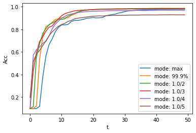
不同的设置可以得到不同的结果,有的推理速度快,但是最终精度低,有的推理慢,但是精度高。用户可以根据自己的需求选择模型设置。
- 1(1,2,3,4,5,6)
Rueckauer B, Lungu I-A, Hu Y, Pfeiffer M and Liu S-C (2017) Conversion of Continuous-Valued Deep Networks to Efficient Event-Driven Networks for Image Classification. Front. Neurosci. 11:682.
- 2
Diehl, Peter U. , et al. Fast classifying, high-accuracy spiking deep networks through weight and threshold balancing. Neural Networks (IJCNN), 2015 International Joint Conference on IEEE, 2015.
- 3
Rueckauer, B., Lungu, I. A., Hu, Y., & Pfeiffer, M. (2016). Theory and tools for the conversion of analog to spiking convolutional neural networks. arXiv preprint arXiv:1612.04052.
- 4
Sengupta, A., Ye, Y., Wang, R., Liu, C., & Roy, K. (2019). Going deeper in spiking neural networks: Vgg and residual architectures. Frontiers in neuroscience, 13, 95.