ANN2SNN
Author: DingJianhao, fangwei123456, Lv Liuzhenghao
This tutorial focuses on spikingjelly.activation_based.ann2snn, introduce how to convert the trained feedforward ANN to SNN and simulate it on the SpikingJelly framework.
ANN2SNN api references are here api references .
There are two sets of implementations in earlier implementations: ONNX-based and PyTorch-based. This version is based on torch.fx. Fx is specially used to transform nn.Module instances, and will natively decouple complex models when building graph intermediate representation. Let’s have a look!
Theoretical basis of ANN2SNN
Compared with ANN, the generated pulses of SNN are discrete, which is conducive to efficient communication. Today, with the popularity of ANN, the direct training of SNN requires more resources.
Naturally, we will think of using the now very mature ANN to convert to SNN, and hope that SNN can have similar performance. This involves the problem of how to build a bridge between ANN and SNN.
Now the mainstream way of SNN is to use frequency encoding, so for the output layer, we will use the number of neuron output pulses to judge the category. Is there a relationship between the release rate and ANN?
Fortunately, there is a strong correlation between the nonlinear activation of ReLU neurons in ANN and the firing rate of IF neurons in SNN (reset by subtracting the threshold \(V_{threshold}\) ). this feature to convert. The neuron update method mentioned here is the Soft method mentioned in Neuron tutorial.
Experiment: Relationship between IF neuron spiking frequency and input
We gave constant input to the IF neuron and observed its output spikes and spike firing frequency. First import the relevant modules, create a new IF neuron layer, determine the input and draw the input of each IF neuron \(x_{i}\):
import torch
from spikingjelly.activation_based import neuron
from spikingjelly import visualizing
from matplotlib import pyplot as plt
import numpy as np

plt.rcParams['figure.dpi'] = 200
if_node = neuron.IFNode(v_reset=None)
T = 128
x = torch.arange(-0.2, 1.2, 0.04)
plt.scatter(torch.arange(x.shape[0]), x)
plt.title('Input $x_{i}$ to IF neurons')
plt.xlabel('Neuron index $i$')
plt.ylabel('Input $x_{i}$')
plt.grid(linestyle='-.')
plt.show()

Next, send the input to the IF neuron layer, and run the T=128 step to observe the pulses and pulse firing frequency of each neuron:
s_list = []
for t in range(T):
    s_list.append(if_node(x).unsqueeze(0))

out_spikes = np.asarray(torch.cat(s_list))
visualizing.plot_1d_spikes(out_spikes, 'IF neurons\' spikes and firing rates', 't', 'Neuron index $i$')
plt.show()

It can be found that the frequency of the pulse firing is within a certain range, which is proportional to the size of the input \(x_{i}\).
Next, let’s plot the firing frequency of the IF neuron against the input \(x_{i}\) and compare it with \(\mathrm{ReLU}(x_{i})\):
plt.subplot(1, 2, 1)
firing_rate = np.mean(out_spikes, axis=1)
plt.plot(x, firing_rate)
plt.title('Input $x_{i}$ and firing rate')
plt.xlabel('Input $x_{i}$')
plt.ylabel('Firing rate')
plt.grid(linestyle='-.')

plt.subplot(1, 2, 2)
plt.plot(x, x.relu())
plt.title('Input $x_{i}$ and ReLU($x_{i}$)')
plt.xlabel('Input $x_{i}$')
plt.ylabel('ReLU($x_{i}$)')
plt.grid(linestyle='-.')
plt.show()

It can be found that the two curves are almost the same. It should be noted that the pulse frequency cannot be higher than 1, so the IF neuron cannot fit the input of the ReLU in the ANN is larger than 1.
Theoretical basis of ANN2SNN
The literature 1 provides a theoretical basis for analyzing the conversion of ANN to SNN. The theory shows that the IF neuron in SNN is an unbiased estimator of ReLU activation function over time.
For the first layer of the neural network, the input layer, discuss the relationship between the firing rate of SNN neurons \(r\) and the activation in the corresponding ANN. Assume that the input is constant as \(z \in [0,1]\). For the IF neuron reset by subtraction, its membrane potential V changes with time as follows:
Where: \(V_{threshold}\) is the firing threshold, usually set to 1.0. \(\theta_t\) is the output spike. The average firing rate in the \(T\) time steps can be obtained by summing the membrane potential:
Move all the items containing \(V_t\) to the left, and divide both sides by \(T\):
Where \(N\) is the number of pulses in the time step of \(T\), and \(\frac{N}{T}\) is the issuing rate \(r\). Use \(z = V_{threshold} a\) which is:
Therefore, when the simulation time step \(T\) is infinite:
Similarly, for the higher layers of the neural network, literature 1 further explains that the inter-layer firing rate satisfies:
For details, please refer to 1. The methods in ann2snn also mainly come from 1 .
Converting to spiking neural network
Conversion mainly solves two problems:
ANN proposes Batch Normalization for fast training and convergence. Batch normalization aims to normalize the ANN output to 0 mean, which is contrary to the properties of SNNs. Therefore, the parameters of BN can be absorbed into the previous parameter layers (Linear, Conv2d)
According to the transformation theory, the input and output of each layer of ANN need to be limited to the range of [0,1], which requires scaling the parameters (model normalization)
◆ BatchNorm parameter absorption
Assume that the parameters of BatchNorm are: math:gamma (BatchNorm.weight), \(\beta\) (BatchNorm.bias), \(\mu\) (BatchNorm. .running_mean) ,
\(\sigma\) (BatchNorm.running_var, \(\sigma = \sqrt{\mathrm{running\_var}}\)). For specific parameter definitions, see
torch.nn.BatchNorm1d .
Parameter modules (eg Linear) have parameters \(W\) and \(b\) . BatchNorm parameter absorption is to transfer the parameters of BatchNorm to \(W\) and \(b\) of the parameter module by operation, so that the output of the new module of data input is the same as when there is BatchNorm.
For this, the \(\bar{W}\) and \(\bar{b}\) formulas for the new model are expressed as:
◆ Model Normalization
For a parameter module, it is assumed that its input tensor and output tensor are obtained, the maximum value of its input tensor is \(\lambda_{pre}\), and the maximum value of its output tensor is \(\lambda\). Then, the normalized weight \(\hat{W}\) is:
The normalized bias \(\hat{b}\) is:
Although the distribution of the output of each layer of ANN obeys a certain distribution, there are often large outliers in the data, which will lead to a decrease in the overall neuron firing rate. To address this, robust normalization adjusts the scaling factor from the maximum value of the tensor to the p-quantile of the tensor. The recommended quantile value in the literature is 99.9.
So far, what we have done with neural networks is numerically equivalent. The current model should perform the same as the original model.
In the conversion, we need to change the ReLU activation function in the original model into IF neurons. For average pooling in ANN, we need to convert it to spatial downsampling. Since IF neurons can be equivalent to the ReLU activation function. Adding IF neurons or not after spatial downsampling has minimal effect on the results. There is currently no very ideal solution for max pooling in ANNs. The best solution so far is to control the pulse channel 1 with a gating function based on momentum accumulated pulses. Here we still recommend using avgpool2d. When simulating, according to the transformation theory, the SNN needs to input a constant analog input. Using a Poisson encoder will bring about a reduction in accuracy.
Implementation and optional configuration
The ann2snn framework was updated in April 2022. The two categories of parser and simulator have been cancelled, and instead the converter class has been used. It is more concise and has more modes for transformation settings.
The framework was updated again in October 2022. Fuse method has benn added to the converter class to fuse the conv layer and the bn layer.
◆ Converter class
This class is used to convert ReLU’s ANN to SNN.
Three common patterns are implemented here:
The most common is the maximum current switching mode (MaxNorm), which utilizes the upper and lower activation limits of the front and rear layers so that the case with the highest firing rate corresponds to the case where the activation achieves the maximum value. Using this mode requires setting the parameter mode to max 2.
The 99.9% current switching mode (RobustNorm) utilizes the 99.9% activation quantile to limit the upper activation limit. Using this mode requires setting the parameter mode to 99.9% 1.
In the scaling conversion mode, the user needs to specify the scaling parameters into the mode, and the current can be limited by the activated maximum value after scaling. Using this mode requires setting the parameter mode to a float of 0-1.
The optional fuse_conv_bn feature is realized:
You can set fuse_flag to True (by default), in order to fuse fuse the conv layer and the bn layer.
After converting, ReLU modules will be removed. And new modules needed by SNN, such as VoltageScaler and IFNode, will be created and stored in the parent module snn tailor.
Due to the type of the return model is fx.GraphModule, you can use ‘print(fx.GraphModule.graph)’ to view how modules links and the how the forward method works. More APIs are here GraphModule .
Classify MNIST
Build the ANN to be converted
Now we use ann2snn to build a simple convolutional network to classify the MNIST dataset.
First define our network structure (see ann2snn.sample_models.mnist_cnn):
class ANN(nn.Module):
    def __init__(self):
        super().__init__()
        self.network = nn.Sequential(
            nn.Conv2d(1, 32, 3, 1),
            nn.BatchNorm2d(32, eps=1e-3),
            nn.ReLU(),
            nn.AvgPool2d(2, 2),

            nn.Conv2d(32, 32, 3, 1),
            nn.BatchNorm2d(32, eps=1e-3),
            nn.ReLU(),
            nn.AvgPool2d(2, 2),

            nn.Conv2d(32, 32, 3, 1),
            nn.BatchNorm2d(32, eps=1e-3),
            nn.ReLU(),
            nn.AvgPool2d(2, 2),

            nn.Flatten(),
            nn.Linear(32, 10),
            nn.ReLU()
        )

    def forward(self,x):
        x = self.network(x)
        return x
Note: If you need to expand the tensor, define a nn.Flatten module in the network, and use the defined Flatten instead of the view function in the forward function.
Define our hyperparameters:
torch.random.manual_seed(0)
torch.cuda.manual_seed(0)
device = 'cuda'
dataset_dir = 'G:/Dataset/mnist'
batch_size = 100
T = 50
Here T is the inference time step used in inference for a while.
If you want to train, you also need to initialize the data loader, optimizer, loss function, for example:
lr = 1e-3
epochs = 10
loss_function = nn.CrossEntropyLoss()
optimizer = torch.optim.Adam(ann.parameters(), lr=lr, weight_decay=5e-4)
Train the ANN. In the example, our model is trained for 10 epochs. The test set accuracy changes during training are as follows:
Epoch: 0 100%|██████████| 600/600 [00:05<00:00, 112.04it/s]
Validating Accuracy: 0.972
Epoch: 1 100%|██████████| 600/600 [00:05<00:00, 105.43it/s]
Validating Accuracy: 0.986
Epoch: 2 100%|██████████| 600/600 [00:05<00:00, 107.49it/s]
Validating Accuracy: 0.987
Epoch: 3 100%|██████████| 600/600 [00:05<00:00, 109.26it/s]
Validating Accuracy: 0.990
Epoch: 4 100%|██████████| 600/600 [00:05<00:00, 103.98it/s]
Validating Accuracy: 0.984
Epoch: 5 100%|██████████| 600/600 [00:05<00:00, 100.42it/s]
Validating Accuracy: 0.989
Epoch: 6 100%|██████████| 600/600 [00:06<00:00, 96.24it/s]
Validating Accuracy: 0.991
Epoch: 7 100%|██████████| 600/600 [00:05<00:00, 104.97it/s]
Validating Accuracy: 0.992
Epoch: 8 100%|██████████| 600/600 [00:05<00:00, 106.45it/s]
Validating Accuracy: 0.991
Epoch: 9 100%|██████████| 600/600 [00:05<00:00, 111.93it/s]
Validating Accuracy: 0.991
After training the model, we quickly load the model to test the performance of the saved model:
model.load_state_dict(torch.load('SJ-mnist-cnn_model-sample.pth'))
acc = val(model, device, test_data_loader)
print('ANN Validating Accuracy: %.4f' % (acc))
The output is as follows:
100%|██████████| 200/200 [00:02<00:00, 89.44it/s]
ANN Validating Accuracy: 0.9870
Make the conversion with the converter
Converting with Converter is very simple, you only need to set the mode you want to use in the parameters. For example, to use MaxNorm, you need to define an ann2snn.Converter first, and forward the model to this object:
model_converter = ann2snn.Converter(mode='max', dataloader=train_data_loader)
snn_model = model_converter(model)
snn_model is the output SNN model. View the network structure of the snn_model (the absence of BatchNorm2d is due to conv_bn_fuse during the conversion process, i.e. absorbing the parameters of the bn layer into the conv layer):
ANN(
  (network): Module(
    (0): Conv2d(1, 32, kernel_size=(3, 3), stride=(1, 1))
    (3): AvgPool2d(kernel_size=2, stride=2, padding=0)
    (4): Conv2d(32, 32, kernel_size=(3, 3), stride=(1, 1))
    (7): AvgPool2d(kernel_size=2, stride=2, padding=0)
    (8): Conv2d(32, 32, kernel_size=(3, 3), stride=(1, 1))
    (11): AvgPool2d(kernel_size=2, stride=2, padding=0)
    (12): Flatten(start_dim=1, end_dim=-1)
    (13): Linear(in_features=32, out_features=10, bias=True)
    (15): Softmax(dim=1)
  )
  (snn tailor): Module(
    (0): Module(
      (0): VoltageScaler(0.240048)
      (1): IFNode(
        v_threshold=1.0, v_reset=None, detach_reset=False, step_mode=s, backend=torch
        (surrogate_function): Sigmoid(alpha=4.0, spiking=True)
      )
      (2): VoltageScaler(4.165831)
    )
    (1): Module(
      (0): VoltageScaler(0.307485)
      (1): IFNode(
        v_threshold=1.0, v_reset=None, detach_reset=False, step_mode=s, backend=torch
        (surrogate_function): Sigmoid(alpha=4.0, spiking=True)
      )
      (2): VoltageScaler(3.252196)
    )
    (2): Module(
      (0): VoltageScaler(0.141659)
      (1): IFNode(
        v_threshold=1.0, v_reset=None, detach_reset=False, step_mode=s, backend=torch
        (surrogate_function): Sigmoid(alpha=4.0, spiking=True)
      )
      (2): VoltageScaler(7.059210)
    )
    (3): Module(
      (0): VoltageScaler(0.060785)
      (1): IFNode(
        v_threshold=1.0, v_reset=None, detach_reset=False, step_mode=s, backend=torch
        (surrogate_function): Sigmoid(alpha=4.0, spiking=True)
      )
      (2): VoltageScaler(16.451399)
    )
  )
)
The type of snn_model is GraphModule , referring to GraphModule .
Call the GraphModule.graph.print_tabular() method to view the graph of the intermediate representation of the model in tabular form:
#snn_model.graph.print_tabular()
opcode       name            target          args               kwargs
-----------  --------------  --------------  -----------------  --------
placeholder  x               x               ()                 {}
call_module  network_0       network.0       (x,)               {}
call_module  snn_tailor_0_1  snn tailor.0.0  (network_0,)       {}
call_module  snn_tailor_0_2  snn tailor.0.1  (snn_tailor_0_1,)  {}
call_module  snn_tailor_0_3  snn tailor.0.2  (snn_tailor_0_2,)  {}
call_module  network_3       network.3       (snn_tailor_0_3,)  {}
call_module  network_4       network.4       (network_3,)       {}
call_module  snn_tailor_1_1  snn tailor.1.0  (network_4,)       {}
call_module  snn_tailor_1_2  snn tailor.1.1  (snn_tailor_1_1,)  {}
call_module  snn_tailor_1_3  snn tailor.1.2  (snn_tailor_1_2,)  {}
call_module  network_7       network.7       (snn_tailor_1_3,)  {}
call_module  network_8       network.8       (network_7,)       {}
call_module  snn_tailor_2_1  snn tailor.2.0  (network_8,)       {}
call_module  snn_tailor_2_2  snn tailor.2.1  (snn_tailor_2_1,)  {}
call_module  snn_tailor_2_3  snn tailor.2.2  (snn_tailor_2_2,)  {}
call_module  network_11      network.11      (snn_tailor_2_3,)  {}
call_module  network_12      network.12      (network_11,)      {}
call_module  network_13      network.13      (network_12,)      {}
call_module  snn_tailor_3_1  snn tailor.3.0  (network_13,)      {}
call_module  snn_tailor_3_2  snn tailor.3.1  (snn_tailor_3_1,)  {}
call_module  snn_tailor_3_3  snn tailor.3.2  (snn_tailor_3_2,)  {}
call_module  network_15      network.15      (snn_tailor_3_3,)  {}
output       output          output          (network_15,)      {}
Comparison of different converting modes
Following this example, we define the modes as max, 99.9% , 1.0/2 , 1.0/3 , 1.0/4 , 1.0/ 5 case SNN transformation and separate inference T steps to get the accuracy.
print('---------------------------------------------')
print('Converting using MaxNorm')
model_converter = ann2snn.Converter(mode='max', dataloader=train_data_loader)
snn_model = model_converter(model)
print('Simulating...')
mode_max_accs = val(snn_model, device, test_data_loader, T=T)
print('SNN accuracy (simulation %d time-steps): %.4f' % (T, mode_max_accs[-1]))

print('---------------------------------------------')
print('Converting using RobustNorm')
model_converter = ann2snn.Converter(mode='99.9%', dataloader=train_data_loader)
snn_model = model_converter(model)
print('Simulating...')
mode_robust_accs = val(snn_model, device, test_data_loader, T=T)
print('SNN accuracy (simulation %d time-steps): %.4f' % (T, mode_robust_accs[-1]))

print('---------------------------------------------')
print('Converting using 1/2 max(activation) as scales...')
model_converter = ann2snn.Converter(mode=1.0 / 2, dataloader=train_data_loader)
snn_model = model_converter(model)
print('Simulating...')
mode_two_accs = val(snn_model, device, test_data_loader, T=T)
print('SNN accuracy (simulation %d time-steps): %.4f' % (T, mode_two_accs[-1]))

print('---------------------------------------------')
print('Converting using 1/3 max(activation) as scales')
model_converter = ann2snn.Converter(mode=1.0 / 3, dataloader=train_data_loader)
snn_model = model_converter(model)
print('Simulating...')
mode_three_accs = val(snn_model, device, test_data_loader, T=T)
print('SNN accuracy (simulation %d time-steps): %.4f' % (T, mode_three_accs[-1]))

print('---------------------------------------------')
print('Converting using 1/4 max(activation) as scales')
model_converter = ann2snn.Converter(mode=1.0 / 4, dataloader=train_data_loader)
snn_model = model_converter(model)
print('Simulating...')
mode_four_accs = val(snn_model, device, test_data_loader, T=T)
print('SNN accuracy (simulation %d time-steps): %.4f' % (T, mode_four_accs[-1]))

print('---------------------------------------------')
print('Converting using 1/5 max(activation) as scales')
model_converter = ann2snn.Converter(mode=1.0 / 5, dataloader=train_data_loader)
snn_model = model_converter(model)
print('Simulating...')
mode_five_accs = val(snn_model, device, test_data_loader, T=T)
print('SNN accuracy (simulation %d time-steps): %.4f' % (T, mode_five_accs[-1]))
Observe the control bar output:
---------------------------------------------
Converting using MaxNorm
100%|██████████| 600/600 [00:04<00:00, 128.25it/s] Simulating...
100%|██████████| 200/200 [00:13<00:00, 14.44it/s] SNN accuracy (simulation 50 time-steps): 0.9777
---------------------------------------------
Converting using RobustNorm
100%|██████████| 600/600 [00:19<00:00, 31.06it/s] Simulating...
100%|██████████| 200/200 [00:13<00:00, 14.75it/s] SNN accuracy (simulation 50 time-steps): 0.9841
---------------------------------------------
Converting using 1/2 max(activation) as scales...
100%|██████████| 600/600 [00:04<00:00, 126.64it/s] ]Simulating...
100%|██████████| 200/200 [00:13<00:00, 14.90it/s] SNN accuracy (simulation 50 time-steps): 0.9844
---------------------------------------------
Converting using 1/3 max(activation) as scales
100%|██████████| 600/600 [00:04<00:00, 126.27it/s] Simulating...
100%|██████████| 200/200 [00:13<00:00, 14.73it/s] SNN accuracy (simulation 50 time-steps): 0.9828
---------------------------------------------
Converting using 1/4 max(activation) as scales
100%|██████████| 600/600 [00:04<00:00, 128.94it/s] Simulating...
100%|██████████| 200/200 [00:13<00:00, 14.47it/s] SNN accuracy (simulation 50 time-steps): 0.9747
---------------------------------------------
Converting using 1/5 max(activation) as scales
100%|██████████| 600/600 [00:04<00:00, 121.18it/s] Simulating...
100%|██████████| 200/200 [00:13<00:00, 14.42it/s] SNN accuracy (simulation 50 time-steps): 0.9487
---------------------------------------------
The speed of model conversion can be seen to be very fast. Model inference speed of 200 steps takes only 11s to complete (GTX 2080ti). Based on the time-varying accuracy of the model output, we can plot the accuracy for different settings.
fig = plt.figure()
plt.plot(np.arange(0, T), mode_max_accs, label='mode: max')
plt.plot(np.arange(0, T), mode_robust_accs, label='mode: 99.9%')
plt.plot(np.arange(0, T), mode_two_accs, label='mode: 1.0/2')
plt.plot(np.arange(0, T), mode_three_accs, label='mode: 1.0/3')
plt.plot(np.arange(0, T), mode_four_accs, label='mode: 1.0/4')
plt.plot(np.arange(0, T), mode_five_accs, label='mode: 1.0/5')
plt.legend()
plt.xlabel('t')
plt.ylabel('Acc')
plt.show()
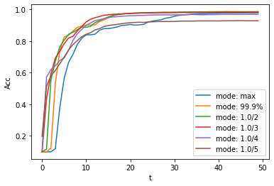
Different settings can get different results, some inference speed is fast, but the final accuracy is low, and some inference is slow, but the accuracy is high. Users can choose model settings according to their needs.
- 1(1,2,3,4,5,6)
Rueckauer B, Lungu I-A, Hu Y, Pfeiffer M and Liu S-C (2017) Conversion of Continuous-Valued Deep Networks to Efficient Event-Driven Networks for Image Classification. Front. Neurosci. 11:682.
- 2
Diehl, Peter U. , et al. Fast classifying, high-accuracy spiking deep networks through weight and threshold balancing. Neural Networks (IJCNN), 2015 International Joint Conference on IEEE, 2015.
- 3
Rueckauer, B., Lungu, I. A., Hu, Y., & Pfeiffer, M. (2016). Theory and tools for the conversion of analog to spiking convolutional neural networks. arXiv preprint arXiv:1612.04052.
- 4
Sengupta, A., Ye, Y., Wang, R., Liu, C., & Roy, K. (2019). Going deeper in spiking neural networks: Vgg and residual architectures. Frontiers in neuroscience, 13, 95.