Basic Conception
Author: fangwei123456
Translator: Qiu Haonan, fangwei123456
This tutorial introduces spikingjelly.activation_based. It is recommended that all users read this tutorial before using SpikingJelly.
Spikingjelly is a deep learning framework for Spiking Neural Network (SNN) based on PyTorch. Users who want to use SpikingJelly should first be familiar with the usage of PyTorch.If the user doesn’t know much about PyTorch, we recommend that the user can learn the basic tutorial of PyTorch first PyTorch Tutorials 。
Activation-based Representation
spikingjelly.activation_based uses tensors whose element is only 0 or 1 to represent spikes. For example:
import torch

v = torch.rand([8])
v_th = 0.5
spike = (v >= v_th).to(v)
print('spike =', spike)
# spike = tensor([0., 0., 0., 1., 1., 0., 1., 0.])
Data Format
In spikingjelly.activation_based, There are two formats of data:
Data in a single time-step with
shape = [N, *], whereNis the batch dimension,*represents any extra dimensions.Data in many time-steps with
shape = [T, N, *], whereTis the time-step dimension,Nis the batch dimension and * represents any additional dimensions.
Step Mode
Modules in spikingjelly.activation_based have two propagation modes, which are the single-step mode ‘s’ and the multi-step mode ‘m’. In single-step mode, the data use the shape = [N, *] format. In multi-step mode, the data use the shape = [T, N, *] format.
The user can set step_mode of a module in its __init__ or change step_mode anytime after the module is built.
import torch
from spikingjelly.activation_based import neuron

net = neuron.IFNode(step_mode='m')
# 'm' is the multi-step mode
net.step_mode = 's'
# 's' is the single-step mode
If we want to input the sequence data with shape = [T, N, *] to a single-step module, we need to implement a for-loop in time-steps manually, which splits the sequence data into T data with shape = [N, *] and sends the data step-by-step. Let’s create a new layer of IF neurons, set it to single-step mode, and input sequence data step-by-step:
import torch
from spikingjelly.activation_based import neuron

net_s = neuron.IFNode(step_mode='s')
T = 4
N = 1
C = 3
H = 8
W = 8
x_seq = torch.rand([T, N, C, H, W])
y_seq = []
for t in range(T):
    x = x_seq[t]  # x.shape = [N, C, H, W]
    y = net_s(x)  # y.shape = [N, C, H, W]
    y_seq.append(y.unsqueeze(0))

y_seq = torch.cat(y_seq)
# y_seq.shape = [T, N, C, H, W]
multi_step_forward wraps the for-loop in time-steps for single-step modules to handle sequence data with shape = [T, N, *], which is more convenient to use:
import torch
from spikingjelly.activation_based import neuron, functional
net_s = neuron.IFNode(step_mode='s')
T = 4
N = 1
C = 3
H = 8
W = 8
x_seq = torch.rand([T, N, C, H, W])
y_seq = functional.multi_step_forward(x_seq, net_s)
# y_seq.shape = [T, N, C, H, W]
However, the best usage is to set the module as a multi-step module directly:
import torch
from spikingjelly.activation_based import neuron

net_m = neuron.IFNode(step_mode='m')
T = 4
N = 1
C = 3
H = 8
W = 8
x_seq = torch.rand([T, N, C, H, W])
y_seq = net_m(x_seq)
# y_seq.shape = [T, N, C, H, W]
To maintain compatibility with codes using older versions of SpikingJelly, the default step mode for all modules in SpikingJelly is single-step.
Saving and Resetting of States
Similar to RNN, neurons and other modules in SNN have hidden states, and their outputs \(Y[t]\) are determined not only by the input :math: X[t] at the current time-step t, but also by the state \(H[t-1]\) at last time-step t-1, which is \(Y[t] = f(X[t], H[t-1])\).
In PyTorch, RNN outputs not only \(Y\) but also \(H\). Refer to torch.nn.RNN for more details. Different from PyTorch, the states are stored inside the module in spikingjelly.activation_based. For example, let us create a new layer of IF neurons, set them to single-step mode, and check the default voltage before and after giving inputs:
import torch
from spikingjelly.activation_based import neuron

net_s = neuron.IFNode(step_mode='s')
x = torch.rand([4])
print(net_s)
print(f'the initial v={net_s.v}')
y = net_s(x)
print(f'x={x}')
print(f'y={y}')
print(f'v={net_s.v}')

# outputs are:

'''
IFNode(
v_threshold=1.0, v_reset=0.0, detach_reset=False
(surrogate_function): Sigmoid(alpha=4.0, spiking=True)
)
the initial v=0.0
x=tensor([0.5543, 0.0350, 0.2171, 0.6740])
y=tensor([0., 0., 0., 0.])
v=tensor([0.5543, 0.0350, 0.2171, 0.6740])
'''
After initialization, the v of the IF neurons layer is set to 0 and is automatically broadcast to have the same shape as the input.
If we give a new input sample, we should clear the previous states of the neurons and reset the neurons to the initialization states, which can be done by calling the module’s self.reset() function:
import torch
from spikingjelly.activation_based import neuron

net_s = neuron.IFNode(step_mode='s')
x = torch.rand([4])
print(f'check point 0: v={net_s.v}')
y = net_s(x)
print(f'check point 1: v={net_s.v}')
net_s.reset()
print(f'check point 2: v={net_s.v}')
x = torch.rand([8])
y = net_s(x)
print(f'check point 3: v={net_s.v}')

# outputs are:

'''
check point 0: v=0.0
check point 1: v=tensor([0.9775, 0.6598, 0.7577, 0.2952])
check point 2: v=0.0
check point 3: v=tensor([0.8728, 0.9031, 0.2278, 0.5089, 0.1059, 0.0479, 0.5008, 0.8530])
'''
For convenience, we can also call spikingjelly.activation_based.functional.reset_net to reset all modules in a network.
If the network uses one or more stateful modules, it must be reset after processing one batch of data during training and inference:
from spikingjelly.activation_based import functional
# ...
for x, label in tqdm(train_data_loader):
    # ...
    optimizer.zero_grad()
    y = net(x)
    loss = criterion(y, label)
    loss.backward()
    optimizer.step()

    functional.reset_net(net)
    # Never forget to reset the network!
If we forget to reset, we may get a wrong output during inference or an error during training:
RuntimeError: Trying to backward through the graph a second time (or directly access saved variables after they have already been freed).
Saved intermediate values of the graph are freed when you call .backward() or autograd.grad().
Specify retain_graph=True if you need to backward through the graph a second time or if you need to access saved variables after calling backward.
Propagation Patterns
If all modules in a network are single-step modules, the computation graph of the entire network is built step-by-step. For example:
for t in range(T):
    x = x_seq[t]
    y = net(x)
    y_seq_step_by_step.append(y.unsqueeze(0))

y_seq_step_by_step = torch.cat(y_seq_step_by_step, 0)
If all modules in a network are multi-step modules, the computation graph of the entire network is built layer-by-layer. For example:
import torch
import torch.nn as nn
from spikingjelly.activation_based import neuron, functional, layer
T = 4
N = 2
C = 8
x_seq = torch.rand([T, N, C]) * 64.

net = nn.Sequential(
    layer.Linear(C, 4),
    neuron.IFNode(),
    layer.Linear(4, 2),
    neuron.IFNode()
)

functional.set_step_mode(net, step_mode='m')
with torch.no_grad():
    y_seq_layer_by_layer = x_seq
    for i in range(net.__len__()):
        y_seq_layer_by_layer = net[i](y_seq_layer_by_layer)
In most cases, we don’t need an explicit implementation of for i in range(net.__len__()), because torch.nn.Sequential has already done that for us. So, we write codes in the following simple style:
y_seq_layer_by_layer = net(x_seq)
The only difference between step-by-step and layer-by-layer is the building order of the computation graph, and their outputs are identical:
import torch
import torch.nn as nn
from spikingjelly.activation_based import neuron, functional, layer
T = 4
N = 2
C = 3
H = 8
W = 8
x_seq = torch.rand([T, N, C, H, W]) * 64.

net = nn.Sequential(
layer.Conv2d(3, 8, kernel_size=3, padding=1, stride=1, bias=False),
neuron.IFNode(),
layer.MaxPool2d(2, 2),
neuron.IFNode(),
layer.Flatten(start_dim=1),
layer.Linear(8 * H // 2 * W // 2, 10),
neuron.IFNode(),
)

print(f'net={net}')

with torch.no_grad():
    y_seq_step_by_step = []
    for t in range(T):
        x = x_seq[t]
        y = net(x)
        y_seq_step_by_step.append(y.unsqueeze(0))

    y_seq_step_by_step = torch.cat(y_seq_step_by_step, 0)
    # we can also use `y_seq_step_by_step = functional.multi_step_forward(x_seq, net)` to get the same results

    print(f'y_seq_step_by_step=\n{y_seq_step_by_step}')

    functional.reset_net(net)
    functional.set_step_mode(net, step_mode='m')
    y_seq_layer_by_layer = net(x_seq)

    max_error = (y_seq_layer_by_layer - y_seq_step_by_step).abs().max()
    print(f'max_error={max_error}')
The outputs of the above codes are:
net=Sequential(
(0): Conv2d(3, 8, kernel_size=(3, 3), stride=(1, 1), padding=(1, 1), bias=False, step_mode=s)
(1): IFNode(
    v_threshold=1.0, v_reset=0.0, detach_reset=False, step_mode=s
    (surrogate_function): Sigmoid(alpha=4.0, spiking=True)
)
(2): MaxPool2d(kernel_size=2, stride=2, padding=0, dilation=1, ceil_mode=False, step_mode=s)
(3): IFNode(
    v_threshold=1.0, v_reset=0.0, detach_reset=False, step_mode=s
    (surrogate_function): Sigmoid(alpha=4.0, spiking=True)
)
(4): Flatten(start_dim=1, end_dim=-1, step_mode=s)
(5): Linear(in_features=128, out_features=10, bias=True)
(6): IFNode(
    v_threshold=1.0, v_reset=0.0, detach_reset=False, step_mode=s
    (surrogate_function): Sigmoid(alpha=4.0, spiking=True)
)
)
y_seq_step_by_step=
tensor([[[0., 0., 0., 0., 0., 0., 0., 0., 0., 0.],
        [0., 0., 0., 0., 0., 0., 0., 0., 0., 0.]],

        [[0., 1., 0., 0., 0., 0., 0., 1., 1., 0.],
        [0., 0., 0., 0., 0., 0., 0., 1., 1., 0.]],

        [[0., 0., 0., 0., 0., 0., 0., 0., 0., 0.],
        [0., 1., 0., 1., 0., 0., 1., 0., 0., 0.]],

        [[0., 1., 0., 0., 0., 0., 1., 0., 1., 0.],
        [0., 0., 0., 0., 0., 0., 0., 1., 1., 0.]]])
max_error=0.0
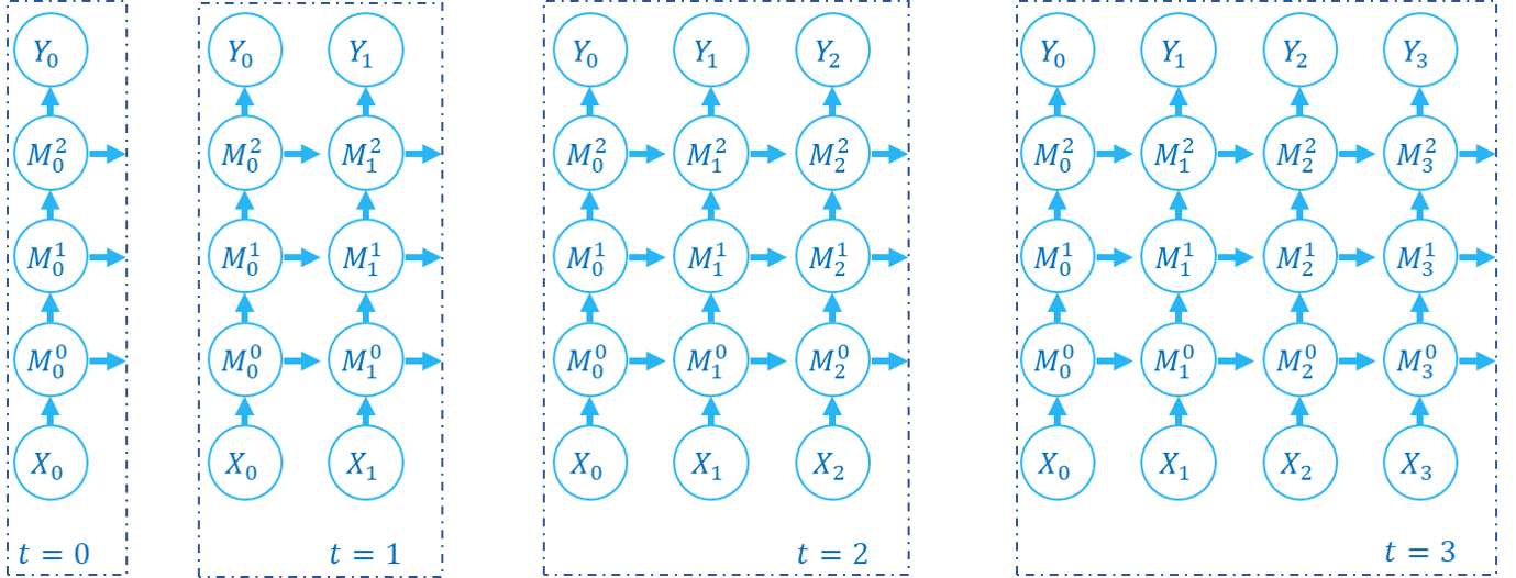
The following figure shows how the computation graph is built in the step-by-step propagation pattern:
The following figure shows how the computation graph is built in the layer-by-layer propagation pattern:
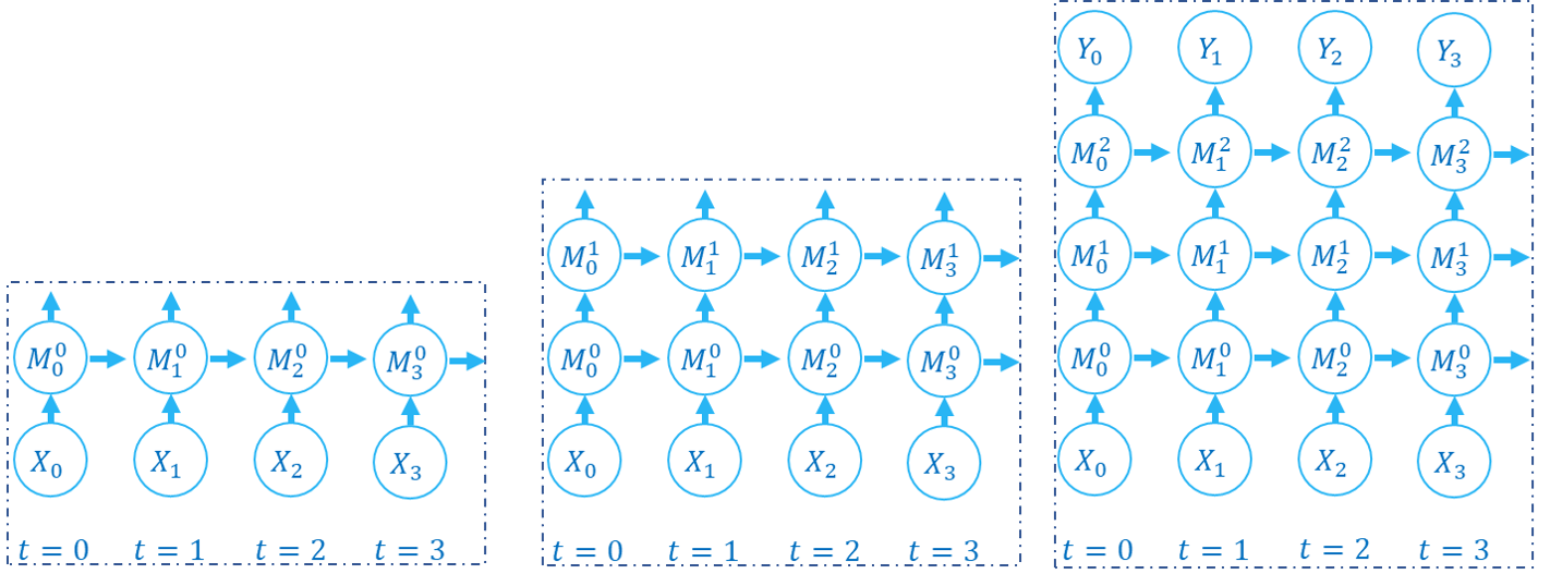
There are two dimensions in the computation graph of SNN, which are the time-step and the depth dimension. As the above figures show, the propagation of SNN is the building of the computation graph.We can find that the step-by-step propagation pattern is a Depth-First-Search (DFS) for traversing the computation graph, while the layer-by-layer propagation pattern is a Breadth-First-Search (BFS) for traversing the computation graph.
Although the difference is only in the building order of the computation graph, there are still some slight differences in computation speed and memory consumption of the two propagation patterns.
When using the surrogate gradient method to train SNN directly, it is recommended to use the layer-by-layer propagation pattern. When the network is built correctly, the layer-by-layer propagation pattern has the advantage of parallelism and speed.
Using step-by-step propagation pattern when memory is limited. For example, a large
Tis required in the ANN2SNN task. In the layer-by-layer propagation pattern, the real batch size for stateless layers isTNrather thanN(refer to the next tutorial). whenTis too large, the memory consumption may be too large.