ANN转换SNN

本页作者：DingJianhao、fangwei123456、Lv Liuzhenghao、黄一凡 (AllenYolk)

English version: ANN2SNN

ANN2SNN 教程导航

当前 ANN2SNN 教程按转换流程拆分：

1. 本页介绍当前 Recipe API 中基于 FX graph 的 rate-coded CNN 转换：RateCodingRecipe / LocalThresholdBalancingRecipe 定义算法，Converter （即 FXConverter 的兼容名）执行转换。

2. Transformer ANN2SNN 转换 介绍面向 Transformer 模型的 STATransformerRecipe 和 SpikeZIPTFQANNRecipe。

旧 API 教程仍可查阅：

1. 更早期 clock-driven 时代 ANN2SNN API。

2. legacy pre-Recipe Converter API，使用 Converter(mode=..., dataloader=...) 和 convert_to_spiking_neurons(model)。

本节介绍 spikingjelly.activation_based.ann2snn，展示如何用当前 Recipe API 将训练好的前馈 ANN 转换为 SNN 并在 SpikingJelly 中仿真。

相关 API 见 API 参考。

本页介绍的 rate-coding 路径基于 torch.fx。torch.fx 会将 nn.Module 实例 trace 为计算图表示，然后由 ANN2SNN FX recipe 对该计算图进行变换。ANN2SNN 也提供不 trace FX graph 的 ModuleConverter，用于 SpikeZIP 这类直接替换 nn.Module tree 的转换；该路径见 Transformer ANN2SNN 教程中的 SpikeZIP 示例。

ANN转换SNN的理论基础

与 ANN 相比，SNN 使用离散脉冲通信，有利于高效计算，但直接训练 SNN 往往需要更多资源。一种做法是先训练 ANN，再将其转换为行为相近的 SNN。这需要建立 ANN 激活值和 SNN 发放率之间的联系。对于 rate-coded SNN，输出类别由脉冲计数读出。核心问题是：脉冲神经元的发放率能否近似 ANN 神经元的激活值？

ANN 中的 ReLU 激活与采用减法重置的 IF 神经元发放率有很强的相关性，其中膜电位会通过减去 \(V_{threshold}\) 重置。这里的神经元更新方式就是 神经元教程 中介绍的 Soft reset 方式。RateCodingRecipe 利用这一关系进行转换。

实验：IF神经元脉冲发放频率和输入的关系

向IF神经元输入恒定值，观察其输出脉冲和脉冲发放频率。先导入模块，创建IF神经元层，画出每个神经元的输入 \(x_{i}\)：

import torch
from spikingjelly.activation_based import neuron
from spikingjelly import visualizing
from matplotlib import pyplot as plt
import numpy as np

plt.rcParams['figure.dpi'] = 200
if_node = neuron.IFNode(v_reset=None)
T = 128
x = torch.arange(-0.2, 1.2, 0.04)
plt.scatter(torch.arange(x.shape[0]), x)
plt.title('Input $x_{i}$ to IF neurons')
plt.xlabel('Neuron index $i$')
plt.ylabel('Input $x_{i}$')
plt.grid(linestyle='-.')
plt.show()

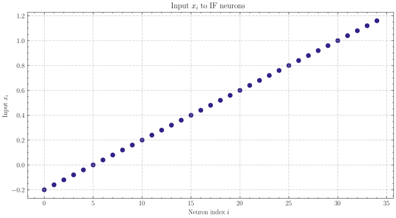
接下来，将输入送入到IF神经元层，并运行 T=128 步，观察各个神经元发放的脉冲、脉冲发放频率：

s_list = []
for t in range(T):
    s_list.append(if_node(x).unsqueeze(0))

out_spikes = np.asarray(torch.cat(s_list))
visualizing.plot_1d_spikes(out_spikes, 'IF neurons\' spikes and firing rates', 't', 'Neuron index $i$')
plt.show()

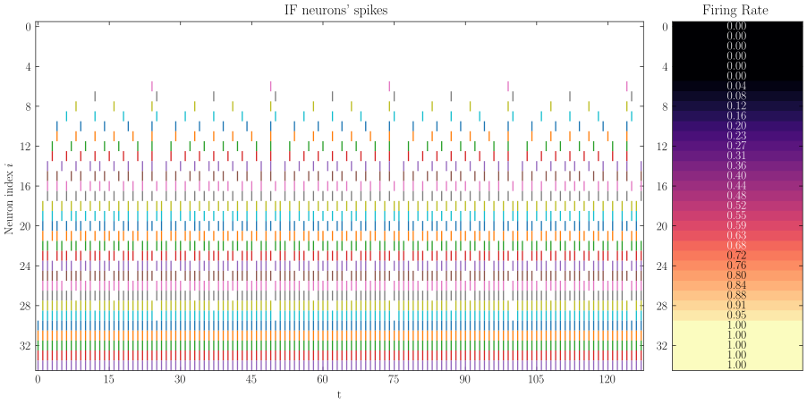
脉冲发放频率在一定范围内与输入 \(x_{i}\) 的大小成正比。

接下来，让我们画出IF神经元脉冲发放频率和输入 \(x_{i}\) 的曲线，并与 \(\mathrm{ReLU}(x_{i})\) 对比：

plt.subplot(1, 2, 1)
firing_rate = np.mean(out_spikes, axis=0)
plt.plot(x, firing_rate)
plt.title('Input $x_{i}$ and firing rate')
plt.xlabel('Input $x_{i}$')
plt.ylabel('Firing rate')
plt.grid(linestyle='-.')

plt.subplot(1, 2, 2)
plt.plot(x, x.relu())
plt.title('Input $x_{i}$ and ReLU($x_{i}$)')
plt.xlabel('Input $x_{i}$')
plt.ylabel('ReLU($x_{i}$)')
plt.grid(linestyle='-.')
plt.show()

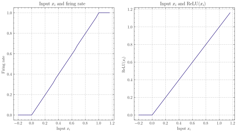
两者的曲线几乎一致。但脉冲频率不可能高于1，因此IF神经元无法拟合ANN中ReLU输入大于1的情况。

理论证明

文献 [1] 为ANN转SNN提供了理论基础，证明SNN中的IF神经元是ReLU激活函数在时间上的无偏估计器。

针对神经网络第一层，考虑 SNN 神经元发放率 \(r\) 和对应 ANN 激活值之间的关系。假定输入恒定为 \(z \in [0,1]\)。对于采用减法重置的IF神经元，其膜电位V随时间变化为：

\[V_t=V_{t-1}+z-V_{threshold}\theta_t\]

其中：

\(V_{threshold}\) 为发放阈值，通常设为1.0。 \(\theta_t\) 为输出脉冲。 \(T\) 时间步内的平均发放率可以通过对膜电位求和得到：

\[\sum_{t=1}^{T} V_t= \sum_{t=1}^{T} V_{t-1}+z T-V_{threshold} \sum_{t=1}^{T}\theta_t\]

将含有 \(V_t\) 的项全部移项到左边，两边同时除以 \(T\) ：

\[\frac{V_T-V_0}{T} = z - V_{threshold} \frac{\sum_{t=1}^{T}\theta_t}{T} = z- V_{threshold} \frac{N}{T}\]

其中 \(N\) 为 \(T\) 时间窗口内的脉冲数， \(\frac{N}{T}\) 就是发放率 \(r\)。利用 \(z= V_{threshold} a\) 即：

\[r = a- \frac{ V_T-V_0 }{T V_{threshold}}\]

故在仿真时间步 \(T\) 无限长情况下:

\[r = a (a>0)\]

类似地，针对神经网络更高层，文献 [1] 进一步说明层间发放率满足：

\[r^l = W^l r^{l-1}+b^l- \frac{V^l_T}{T V_{threshold}}\]

完整推导见文献 [1]。ann2snn 中的方法基于该文献。

转换到脉冲神经网络

转换主要解决两个问题：

1. ANN 使用批归一化（Batch Normalization）加速训练和收敛。批归一化将激活值归一化到零均值，与 SNN 特性冲突。解决方法是将 BN 参数吸收到前面的参数层中（Linear、Conv2d）。

2. 按转换理论，ANN 每层的输入输出需要限制在 [0,1] 范围内，需要对参数进行缩放（模型归一化）。

◆ BatchNorm参数吸收

假定BatchNorm的参数为 \(\gamma\) (BatchNorm.weight)， \(\beta\) (BatchNorm.bias)， \(\mu\) (BatchNorm.running_mean)， \(\sigma\) (BatchNorm.running_var，\(\sigma = \sqrt{\mathrm{running\_var}}\))。具体参数定义详见 torch.nn.BatchNorm1d。参数模块（例如 Linear）具有权重 \(W\) 和偏置 \(b\)。BatchNorm 参数吸收就是将 BatchNorm 的参数通过运算转移到参数模块的 \(W\) 和 \(b\) 中，使得数据输入新模块的输出和有 BatchNorm 时相同。对此，新模型的 \(\bar{W}\) 和 \(\bar{b}\) 公式表示为：

\[\bar{W} = \frac{\gamma}{\sigma} W\]

\[\bar{b} = \frac{\gamma}{\sigma} (b - \mu) + \beta\]

◆ 模型归一化

对于某个参数模块，假定得到了其输入张量和输出张量，其输入张量的最大值为 \(\lambda_{pre}\) ,输出张量的最大值为 \(\lambda\) 那么，归一化后的权重 \(\hat{W}\) 为：

\[\hat{W} = W * \frac{\lambda_{pre}}{\lambda}\]

归一化后的偏置 \(\hat{b}\) 为：

\[\hat{b} = \frac{b}{\lambda}\]

ANN每层输出中常常存在较大的离群值，导致整体神经元发放率降低。鲁棒归一化将缩放因子从张量最大值改为张量的p分位点，推荐分位点为99.9% [1]。

BatchNorm 融合和模型归一化是在脉冲替换前进行的代数变换。随后 rate-coding recipe 会将 ReLU 激活替换为 IF 神经元。对于 ANN 中的平均池化，转换后的模型保留空间下采样。由于 IF 神经元会在时间上近似 ReLU 激活，在空间下采样后立即再增加一个 IF 神经元通常对结果影响很小。当前 rate-coding recipe 没有通用的最大池化转换规则。文献中使用基于动量累计脉冲的门控函数控制脉冲通道 [1]。因此，本教程的示例模型仍推荐使用 AvgPool2d。仿真时，依照该转换理论，转换后的 SNN 应输入恒定的模拟输入。使用 Poisson 编码器可能引入额外的准确率损失。

实现与可选配置

当前 ann2snn API 将算法定义和执行流程分离。对于本页的 rate-coding CNN 转换，使用 FX 路径：

• FXConversionRecipe 持有算法参数和算法相关的图变换。兼容名 ConversionRecipe 等价于 FXConversionRecipe。

• FXConverter 是执行器。兼容名 Converter 等价于 FXConverter。它接收 FX recipe，用 torch.fx trace 模型，并通过 convert(model) 依次调用 recipe 的 FX 转换步骤。

• 直接 nn.Module tree 转换使用 ModuleConversionRecipe 和 ModuleConverter，不执行 FX tracing，也不会由 Converter 自动分发。

如果要做 ReLU-to-IFNode 的 rate-coding 转换，使用 RateCodingRecipe。该 recipe 需要校准 dataloader，因为它会在替换 ReLU 前统计激活范围。常见模式包括：

• mode="max"：MaxNorm，使用最大激活值 [2]。

• mode="99.9%"：RobustNorm，使用 99.9% 激活分位点 [1]。

• mode 为 (0, 1] 内的浮点数：按该比例缩放最大激活值。

RateCodingRecipe 也持有 fuse_flag 等选项。当 fuse_flag=True （默认值）时，Conv-BatchNorm 会在校准前被融合。

最简单的 rate-coding 调用如下：

recipe = ann2snn.RateCodingRecipe(dataloader=train_loader, mode="max")
snn = ann2snn.Converter(recipe=recipe).convert(ann)

转换产物的运行方式与 spikingjelly.activation_based 中其他模块一致。单步模式下，用户显式编写时间循环。Rate-coding 和 LTB 模型在每个时间步接收同一个静态 ANN 输入：

from spikingjelly.activation_based import functional

functional.set_step_mode(snn, "s")
functional.reset_net(snn)

y = None
for t in range(T):
    y_t = snn(x)
    y = y_t if y is None else y + y_t

如果要运行 layer-wise 多步路径，输入第 0 维为时间维的序列，并显式做累计读出：

functional.set_step_mode(snn, "m")
functional.reset_net(snn)

x_seq = x.unsqueeze(0).expand(T, *x.shape)
y_seq = snn(x_seq)
y = y_seq.sum(dim=0)

转换后 ReLU 模块被删除，SNN 需要的新模块（包括 VoltageScaler、IFNode 等）会作为 spiking_* 子模块创建在原父模块下。使用 RateCodingRecipe 时，转换后模型的类型为 fx.GraphModule，所以可以使用 snn.graph.print_tabular() 查看生成的计算图。更多 API 参见 GraphModule。

备注

本页的 FX 转换使用 Converter(recipe=...) 和 Converter.convert(model)。Converter 是 FXConverter 的兼容名，只接受 FXConversionRecipe / ConversionRecipe。旧的公开函数已移除，包括 convert_to_spiking_neurons()、replace_by_td_operators()、fuse()、set_voltagehook()、replace_by_neurons() 和 replace_by_ifnode()。

识别MNIST

构建并加载 ANN

下面用 ann2snn 搭建一个简单卷积网络，对 MNIST 数据集进行分类。

完整的可运行示例是 spikingjelly.activation_based.ann2snn.examples.cnn_mnist。网络结构定义在 ann2snn.sample_models.mnist_cnn 中：

class CNN(nn.Module):
    def __init__(self):
        super().__init__()
        self.network = nn.Sequential(
            nn.Conv2d(1, 32, 3, 1),
            nn.BatchNorm2d(32),
            nn.ReLU(),
            nn.AvgPool2d(2, 2),

            nn.Conv2d(32, 32, 3, 1),
            nn.BatchNorm2d(32),
            nn.ReLU(),
            nn.AvgPool2d(2, 2),

            nn.Conv2d(32, 32, 3, 1),
            nn.BatchNorm2d(32),
            nn.ReLU(),
            nn.AvgPool2d(2, 2),

            nn.Flatten(),
            nn.Linear(32, 10),
        )

    def forward(self, x):
        x = self.network(x)
        return x

注意：如果需要展开 tensor，在网络中定义 nn.Flatten 模块，在 forward 中调用它，而不是使用 view。

定义基本运行选项：

torch.random.manual_seed(0)
if torch.cuda.is_available():
    torch.cuda.manual_seed(0)
device = "cuda" if torch.cuda.is_available() else "cpu"
dataset_dir = "./data/mnist"
batch_size = 100
T = 50

T 是 SNN 推理时使用的仿真步数。转换前先创建 MNIST dataloader：

train_data_dataset = torchvision.datasets.MNIST(
    root=dataset_dir,
    train=True,
    transform=torchvision.transforms.ToTensor(),
    download=True,
)
train_data_loader = torch.utils.data.DataLoader(
    dataset=train_data_dataset, batch_size=batch_size, shuffle=True, drop_last=False
)
calibration_data_loader = torch.utils.data.DataLoader(
    dataset=train_data_dataset, batch_size=batch_size, shuffle=False, drop_last=False
)
test_data_dataset = torchvision.datasets.MNIST(
    root=dataset_dir,
    train=False,
    transform=torchvision.transforms.ToTensor(),
    download=True,
)
test_data_loader = torch.utils.data.DataLoader(
    dataset=test_data_dataset, batch_size=50, shuffle=True, drop_last=False
)

示例脚本会下载预训练 checkpoint。入口函数 download_checkpoint 封装了下载逻辑，download_url 失败时回退到 requests 流式下载。先加载并验证 ANN：

from spikingjelly.activation_based.ann2snn.examples.cnn_mnist import (
    DEFAULT_CHECKPOINT_PATH,
    DEFAULT_CHECKPOINT_URL,
    download_checkpoint,
)
from spikingjelly.activation_based.ann2snn.sample_models import mnist_cnn

download_checkpoint(DEFAULT_CHECKPOINT_URL, DEFAULT_CHECKPOINT_PATH)
model = mnist_cnn.CNN().to(device)
model.load_state_dict(torch.load(DEFAULT_CHECKPOINT_PATH, map_location=device))
acc = val(model, device, test_data_loader)
print('ANN Validating Accuracy: %.4f' % (acc))

本次运行中，ANN 准确率为：

ANN Validating Accuracy: 0.9870

使用Converter进行转换

ANN 训练完成。选择 rate-coding recipe，传入确定性校准 dataloader，由 Converter 执行转换：

recipe = ann2snn.RateCodingRecipe(dataloader=calibration_data_loader, mode="max")
model_converter = ann2snn.Converter(recipe=recipe)
snn_model = model_converter.convert(model)

snn_model 即转换后的 SNN 模型。查看其网络结构，BatchNorm2d 模块已消失——默认 rate-coding recipe 在校准前将 BatchNorm 参数吸收进了前面的 Conv 层：

CNN(
  (network): Module(
    (0): Conv2d(1, 32, kernel_size=(3, 3), stride=(1, 1))
    (3): AvgPool2d(kernel_size=2, stride=2, padding=0)
    (4): Conv2d(32, 32, kernel_size=(3, 3), stride=(1, 1))
    (7): AvgPool2d(kernel_size=2, stride=2, padding=0)
    (8): Conv2d(32, 32, kernel_size=(3, 3), stride=(1, 1))
    (11): AvgPool2d(kernel_size=2, stride=2, padding=0)
    (12): Flatten(start_dim=1, end_dim=-1)
    (13): Linear(in_features=32, out_features=10, bias=True)
    (spiking_0): Module(
      (scaler0): VoltageScaler(0.193247)
      (if_node): IFNode(
        v_threshold=1.0, v_reset=None, detach_reset=False, step_mode=s, backend=torch
        (surrogate_function): Sigmoid(alpha=4.0, spiking=True)
      )
      (scaler1): VoltageScaler(5.174733)
    )
    (spiking_1): Module(
      (scaler0): VoltageScaler(0.325697)
      (if_node): IFNode(
        v_threshold=1.0, v_reset=None, detach_reset=False, step_mode=s, backend=torch
        (surrogate_function): Sigmoid(alpha=4.0, spiking=True)
      )
      (scaler1): VoltageScaler(3.070336)
    )
    (spiking_2): Module(
      (scaler0): VoltageScaler(0.121967)
      (if_node): IFNode(
        v_threshold=1.0, v_reset=None, detach_reset=False, step_mode=s, backend=torch
        (surrogate_function): Sigmoid(alpha=4.0, spiking=True)
      )
      (scaler1): VoltageScaler(8.198915)
    )
  )
)

使用 RateCodingRecipe 时，snn_model 的类型为 GraphModule。可参考 GraphModule。

调用 GraphModule.graph.print_tabular() 可以表格形式查看计算图的中间表示：

# snn_model.graph.print_tabular()
opcode       name                       target                     args                          kwargs
-----------  -------------------------  -------------------------  ----------------------------  ------
placeholder  x                          x                          ()                            {}
call_module  network_0                  network.0                  (x,)                          {}
call_module  network_spiking_0_scaler0  network.spiking_0.scaler0  (network_0,)                  {}
call_module  network_spiking_0_if_node  network.spiking_0.if_node  (network_spiking_0_scaler0,)  {}
call_module  network_spiking_0_scaler1  network.spiking_0.scaler1  (network_spiking_0_if_node,)  {}
call_module  network_3                  network.3                  (network_spiking_0_scaler1,)  {}
call_module  network_4                  network.4                  (network_3,)                  {}
call_module  network_spiking_1_scaler0  network.spiking_1.scaler0  (network_4,)                  {}
call_module  network_spiking_1_if_node  network.spiking_1.if_node  (network_spiking_1_scaler0,)  {}
call_module  network_spiking_1_scaler1  network.spiking_1.scaler1  (network_spiking_1_if_node,)  {}
call_module  network_7                  network.7                  (network_spiking_1_scaler1,)  {}
call_module  network_8                  network.8                  (network_7,)                  {}
call_module  network_spiking_2_scaler0  network.spiking_2.scaler0  (network_8,)                  {}
call_module  network_spiking_2_if_node  network.spiking_2.if_node  (network_spiking_2_scaler0,)  {}
call_module  network_spiking_2_scaler1  network.spiking_2.scaler1  (network_spiking_2_if_node,)  {}
call_module  network_11                 network.11                 (network_spiking_2_scaler1,)  {}
call_module  network_12                 network.12                 (network_11,)                 {}
call_module  network_13                 network.13                 (network_12,)                 {}
output       output                     output                     (network_13,)                 {}

其它 recipe 与自定义 recipe

上面的 MNIST 示例使用 rate coding 将 ReLU 激活转换为 IF 神经元。对于 Transformer 模型，可以改用 TransformerTDEquivalentRecipe：

recipe = ann2snn.TransformerTDEquivalentRecipe()
td_model = ann2snn.Converter(recipe=recipe).convert(transformer_ann)

该 recipe 不需要 dataloader，不插入 VoltageHook，也不运行 rate-coding 校准。它将当前支持的 ANN 模块和 attention 调用替换为 TD-equivalent 算子，但不覆盖完整的 fully spike-driven LLM 转换。在这些 TD 算子中，ann_forward(...) 是普通无状态 PyTorch 路径；single_step_forward(...) 是有状态 temporal-difference 单步传播，处理独立序列前应先 reset()。

要添加新的 FX graph 转换算法，继承 FXConversionRecipe （或兼容名 ConversionRecipe）并覆盖需要改变的步骤方法即可。未覆盖的方法使用基类的默认 no-op 实现。Recipe 不是执行器，不应提供 convert()、run() 或 __call__()：

class MyFXRecipe(ann2snn.FXConversionRecipe):
    def replace(self, converter, fx_model):
        # Implement the algorithm-specific graph rewrite here.
        return fx_model

FX 路径固定步骤顺序为 validate -> before_trace -> after_trace -> insert_observers -> calibrate -> replace -> finalize。

如果算法不需要 FX graph，而是直接替换 nn.Module tree，应继承 ModuleConversionRecipe 并用 ModuleConverter 执行。该路径只有 validate -> convert_module 两步，不存在 before_trace 或 finalize：

class MyModuleRecipe(ann2snn.ModuleConversionRecipe):
    def convert_module(self, converter, ann):
        # Replace submodules in ann or return a converted copy.
        return ann

converted = ann2snn.ModuleConverter(recipe=MyModuleRecipe()).convert(ann)

自定义转换规则

默认情况下，RateCodingRecipe 使用 ReLURule 将 nn.ReLU 模块替换为 VoltageScaler(1 / s) -> IFNode -> VoltageScaler(s)。其中校准尺度 s 由 ThresholdOptimizer 基于 VoltageHook 计算得到。

高级用户可以向 RateCodingRecipe 显式传入以下扩展点：

• rules 负责匹配 FX 计算图节点、插入校准 hook、查找完成校准的activation-hook 节点对，并把它们替换为 SNN 子图。

• NeuronFactory 负责创建替换时使用的神经元。默认工厂创建 IFNode(v_threshold=1.0, v_reset=None)。

• ThresholdOptimizer 负责从已校准的 VoltageHook 计算有限正标量阈值。

下面的最小规则只演示协议形状，不表示新的转换算法。它匹配 nn.Identity，并将完成校准的 identity 节点替换为另一个 nn.Identity 模块：

import torch
import torch.nn as nn

from spikingjelly.activation_based import ann2snn
from spikingjelly.activation_based.ann2snn.modules import VoltageHook


class IdentityRule:
    def match(self, node, modules):
        return node.op == "call_module" and type(modules[node.target]) is nn.Identity

    def insert_hooks(self, fx_model, node, hook_factory, hook_counts_per_prefix):
        target = f'{node.target}_voltage_hook'
        fx_model.add_submodule(target, hook_factory.create())
        with fx_model.graph.inserting_after(node):
            return fx_model.graph.call_module(target, args=(node,))

    def find_replacements(self, fx_model, modules):
        for hook_node in fx_model.graph.nodes:
            if hook_node.op == "call_module" and isinstance(
                modules.get(hook_node.target), VoltageHook
            ):
                yield hook_node.args[0], hook_node

    def replace_with_neurons(
        self, fx_model, activation_node, hook_node, neuron_factory, threshold_optimizer
    ):
        hook = fx_model.get_submodule(hook_node.target)
        threshold = threshold_optimizer.compute_threshold(hook)
        # IdentityRule 不使用脉冲阈值，但真实规则应将该标量接入替换子图。
        target = f'{activation_node.target}_spiking_identity'
        fx_model.add_submodule(target, nn.Identity())
        with fx_model.graph.inserting_after(hook_node):
            new_node = fx_model.graph.call_module(target, args=activation_node.args)
        hook_node.replace_all_uses_with(new_node)
        activation_node.replace_all_uses_with(new_node)
        fx_model.graph.erase_node(hook_node)
        fx_model.graph.erase_node(activation_node)


recipe = ann2snn.RateCodingRecipe(
    dataloader=[torch.randn(2, 4)],
    rules=[IdentityRule()],
)
converter = ann2snn.Converter(recipe=recipe)

当前内置 ReLURule 路径只对标量阈值有明确语义。Per-channel 或张量阈值还需要先定义 shape、broadcast 和 VoltageScaler 语义，不属于当前转换路径。

不同转换模式的对比

按照这个例子，也可以比较 RateCodingRecipe 中不同归一化模式的时间步收敛曲线。完整示例脚本保留了这一旧实验，可以用 --plot-mode-sweep 运行：

python -m spikingjelly.activation_based.ann2snn.examples.cnn_mnist \
  --time-steps 50 \
  --plot-mode-sweep

以下输出是在 NVIDIA GeForce RTX 4090 上以 T=50 测得：

ANN Validating Accuracy: 0.9870
---------------------------------------------
Converting using MaxNorm
Calibration: 3.76s
Simulating...
Simulation: 7.61s
SNN accuracy (simulation 50 time-steps): 0.9771
---------------------------------------------
Converting using RobustNorm
Calibration: 12.08s
Simulating...
Simulation: 7.31s
SNN accuracy (simulation 50 time-steps): 0.9848
---------------------------------------------
Converting using 1/2 max(activation) as scales
Calibration: 3.73s
Simulating...
Simulation: 7.28s
SNN accuracy (simulation 50 time-steps): 0.9846
---------------------------------------------
Converting using 1/3 max(activation) as scales
Calibration: 3.72s
Simulating...
Simulation: 7.29s
SNN accuracy (simulation 50 time-steps): 0.9825
---------------------------------------------
Converting using 1/4 max(activation) as scales
Calibration: 3.75s
Simulating...
Simulation: 7.27s
SNN accuracy (simulation 50 time-steps): 0.9734
---------------------------------------------
Converting using 1/5 max(activation) as scales
Calibration: 3.70s
Simulating...
Simulation: 7.26s
SNN accuracy (simulation 50 time-steps): 0.9472

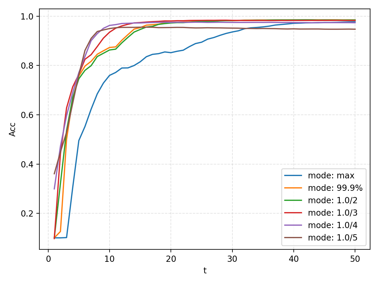
不同归一化模式在早期时间步收敛速度和最终准确率之间形成取舍，可根据延迟和准确率需求选择。

转换 recipe 对比

除了基础的 RateCodingRecipe，SpikingJelly 还提供 LocalThresholdBalancingRecipe，用于在转换阶段估计局部阈值。该 recipe 参考 local threshold balancing 方法 [3]。下面比较 ANN、legacy 标量阈值 RobustNorm 转换和 LTB recipe。完整可运行入口仍是 spikingjelly.activation_based.ann2snn.examples.cnn_mnist：

python -m spikingjelly.activation_based.ann2snn.examples.cnn_mnist \
  --time-steps 32 \
  --output /tmp/ann2snn_mnist_t32.json

下表可以由该命令直接生成。其中 RobustNorm 使用 RateCodingRecipe(dataloader=..., mode="99.9%")。 LTB 使用 LocalThresholdBalancingRecipe(dataloader=..., time_steps=32, mode="99.9%")。本次 MNIST 结果使用完整训练集 60000 张样本作为校准集，使用完整测试集 10000 张样本评估：

MNIST CNN 转换结果

方法	校准样本	测试样本	时间步	Top-1 (%)
ANN		10000		98.70
RobustNorm（legacy，标量阈值）	60000	10000	32	98.35
LocalThresholdBalancingRecipe	60000	10000	32	98.53

ResNet-18 转换

为了展示同一套 recipe 在更大规模模型上的行为，可以运行 ImageNet ResNet-18 示例。该脚本使用 torchvision 的 ResNet18_Weights.IMAGENET1K_V1 权重和对应预处理。校准集为 ImageNet 训练集中的确定性 50000 张子集，评估集为完整 ImageNet 验证集 50000 张。示例命令假设 /path/to/imagenet 下包含 train/ 和 val/ 两个目录；如果数据集组织在额外的 ILSVRC2012/ 等子目录下，请将 --data-root 指向真正包含这两个目录的位置。

备注

SpikingJelly 中的 LocalThresholdBalancingRecipe 是在当前 ANN2SNN recipe 框架内对 local threshold balancing 主要思想的工程化实现，并不是 LTB 原文 [3] 完整 pipeline 的复现。部分论文中特定的工程细节和评测设置没有纳入当前实现。因此，下表中的精度应理解为 SpikingJelly 该 recipe 实现的结果，不能直接视为 LTB 原文方法的官方精度，也不应与论文结果直接对比。

复现命令如下：

CUDA_VISIBLE_DEVICES=0 python -m spikingjelly.activation_based.ann2snn.examples.imagenet_resnet18_ltb \
  --data-root /path/to/imagenet \
  --calib-samples 50000 \
  --batch-size 128 \
  --num-workers 8 \
  --device cuda:0 \
  --time-steps 32 \
  --recipes ann robust_legacy ltb \
  --delay-start auto \
  --output /tmp/ann2snn_imagenet_t32_delayauto_calib50k_tutorial.json

命令中的 robust_legacy 对应不启用 channel_wise 和 half_threshold 的 legacy 标量阈值 RateCodingRecipe。--delay-start auto 会在评估前估计 delayed readout 的起始时间步，用于跳过 SNN 早期 transient。该设置只影响读出窗口，不改变转换后的神经元动力学。下表中的 LTB 完整运行自动估计的 delay_start 为 27；该值依赖模型、校准数据和实现细节，用户运行时可能得到不同数值。

ImageNet ResNet-18 转换结果

方法	校准样本	验证样本	时间步	Top-1 (%)	Top-5 (%)
ANN		50000		69.756	89.074
RobustNorm（legacy，标量阈值）	50000	50000	32	12.462	28.662
LocalThresholdBalancingRecipe	50000	50000	32	65.472	86.636

在较深的 ImageNet CNN 上，缺少 per-channel 归一化的标量阈值 robust normalization 转换精度较低（Top-1 仅 12.462%）。LTB recipe 通过局部阈值估计将 Top-1 提升至 65.472%。

[1] (1,2,3,4,5,6)

Rueckauer B, Lungu I-A, Hu Y, Pfeiffer M and Liu S-C (2017) Conversion of Continuous-Valued Deep Networks to Efficient Event-Driven Networks for Image Classification. Front. Neurosci. 11:682.

[2]

Diehl, Peter U. , et al. Fast classifying, high-accuracy spiking deep networks through weight and threshold balancing. Neural Networks (IJCNN), 2015 International Joint Conference on IEEE, 2015.

[3] (1,2)

Bu T, Li M, Yu Z. Inference-Scale Complexity in ANN-SNN Conversion for High-Performance and Low-Power Applications. arXiv:2409.03368, 2024. Accepted by CVPR 2025.

其他参考文献：

• Rueckauer, B., Lungu, I. A., Hu, Y., & Pfeiffer, M. (2016). Theory and tools for the conversion of analog to spiking convolutional neural networks. arXiv preprint arXiv:1612.04052.

• Sengupta, A., Ye, Y., Wang, R., Liu, C., & Roy, K. (2019). Going deeper in spiking neural networks: Vgg and residual architectures. Frontiers in neuroscience, 13, 95.