ANN2SNN

Author: DingJianhao, fangwei123456, Lv Liuzhenghao, Yifan Huang (AllenYolk)

中文版：ANN转换SNN

ANN2SNN tutorial map

Current ANN2SNN tutorials are split by conversion workflow:

1. This page covers the current FX graph Recipe API for rate-coded CNN conversion: RateCodingRecipe / LocalThresholdBalancingRecipe define the algorithm, and Converter (the compatibility name for FXConverter) executes it.

2. Transformer ANN2SNN conversion covers STATransformerRecipe and SpikeZIPTFQANNRecipe for Transformer models.

Legacy API tutorials remain available:

1. Older clock-driven-era ANN2SNN API.

2. Legacy pre-Recipe Converter API, which used Converter(mode=..., dataloader=...) and convert_to_spiking_neurons(model).

This tutorial focuses on spikingjelly.activation_based.ann2snn. It shows how to convert a trained feedforward ANN to an SNN using the Recipe API and simulate the result.

ANN2SNN API references are available here.

The rate-coding path covered on this page is based on torch.fx. torch.fx traces nn.Module instances into a graph representation, which is then transformed by ANN2SNN FX recipes. ANN2SNN also provides ModuleConverter for conversions that directly replace an nn.Module tree without FX tracing, such as SpikeZIP; see the SpikeZIP section in the Transformer ANN2SNN tutorial for that path.

Theoretical basis of ANN2SNN

SNNs communicate with discrete spikes, which enables efficient event-driven computation, but direct SNN training often requires more resources than ANN training. One approach is to train an ANN first, then convert it to an SNN with similar behavior. For rate-coded SNNs, output classes are read from spike counts. The key question is whether a spiking neuron's firing rate can approximate an ANN neuron's activation.

ReLU activations in ANNs are strongly related to the firing rates of IF neurons with subtractive reset, where the membrane voltage is reset by subtracting \(V_{threshold}\). This neuron update method is the Soft reset method described in the Neuron tutorial. RateCodingRecipe uses this relationship for conversion.

Experiment: Relationship between IF neuron spiking frequency and input

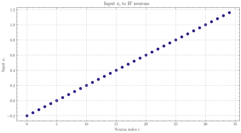
Apply constant input to an IF neuron and observe its output spikes and firing rate. First import the modules, create an IF neuron layer, and plot the input \(x_{i}\) for each neuron:

import torch
from spikingjelly.activation_based import neuron
from spikingjelly import visualizing
from matplotlib import pyplot as plt
import numpy as np

plt.rcParams['figure.dpi'] = 200
if_node = neuron.IFNode(v_reset=None)
T = 128
x = torch.arange(-0.2, 1.2, 0.04)
plt.scatter(torch.arange(x.shape[0]), x)
plt.title('Input $x_{i}$ to IF neurons')
plt.xlabel('Neuron index $i$')
plt.ylabel('Input $x_{i}$')
plt.grid(linestyle='-.')
plt.show()

Send the input to the IF neuron layer for T=128 steps and observe the output spikes and firing rates:

s_list = []
for t in range(T):
    s_list.append(if_node(x).unsqueeze(0))

out_spikes = np.asarray(torch.cat(s_list))
visualizing.plot_1d_spikes(out_spikes, 'IF neurons\' spikes and firing rates', 't', 'Neuron index $i$')
plt.show()

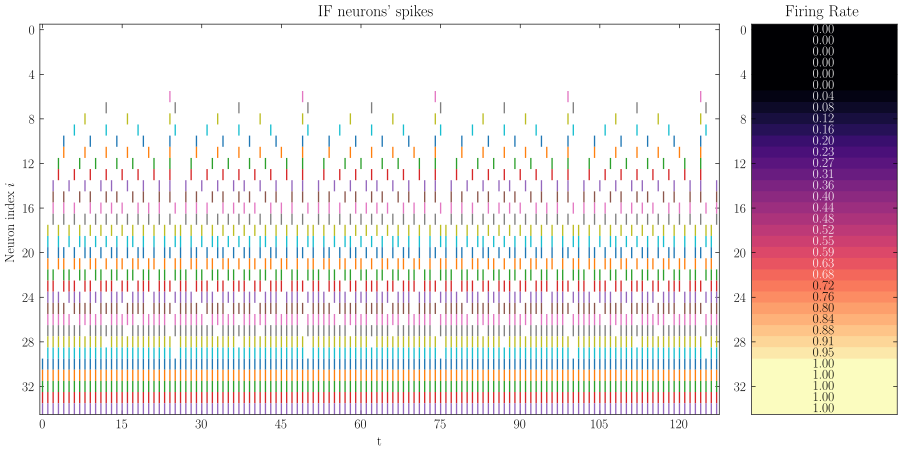
Within a certain range, the firing frequency is proportional to the input \(x_{i}\).

Plot the firing rate against the input \(x_{i}\) and compare it with \(\mathrm{ReLU}(x_{i})\):

plt.subplot(1, 2, 1)
firing_rate = np.mean(out_spikes, axis=0)
plt.plot(x, firing_rate)
plt.title('Input $x_{i}$ and firing rate')
plt.xlabel('Input $x_{i}$')
plt.ylabel('Firing rate')
plt.grid(linestyle='-.')

plt.subplot(1, 2, 2)
plt.plot(x, x.relu())
plt.title('Input $x_{i}$ and ReLU($x_{i}$)')
plt.xlabel('Input $x_{i}$')
plt.ylabel('ReLU($x_{i}$)')
plt.grid(linestyle='-.')
plt.show()

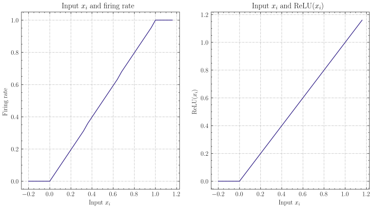
The two curves are nearly identical. However, the firing rate cannot exceed 1, so the IF neuron cannot approximate ReLU activations larger than 1.

Theoretical proof

Literature [1] provides an analytical basis for ANN-to-SNN conversion. The theory shows that an IF neuron in an SNN is an unbiased estimator of the ReLU activation over time.

Consider the first layer. Let the firing rate of SNN neurons be \(r\) and the corresponding ANN activation be \(a\). Assume constant input \(z \in [0,1]\). For an IF neuron with subtractive reset, the membrane potential evolves as:

\[V_t=V_{t-1}+z-V_{threshold}\theta_t\]

where \(V_{threshold}\) is the firing threshold (usually 1.0) and \(\theta_t\) is the output spike. The average firing rate over \(T\) steps can be derived by summing the membrane potential:

\[\sum_{t=1}^{T} V_t= \sum_{t=1}^{T} V_{t-1}+z T-V_{threshold} \sum_{t=1}^{T}\theta_t\]

Rearranging the \(V_t\) terms and dividing by \(T\):

\[\frac{V_T-V_0}{T} = z - V_{threshold} \frac{\sum_{t=1}^{T}\theta_t}{T} = z- V_{threshold} \frac{N}{T}\]

where \(N\) is the spike count in the time window \(T\), and \(\frac{N}{T}\) is the firing rate \(r\). Substituting \(z = V_{threshold} a\):

\[r = a- \frac{ V_T-V_0 }{T V_{threshold}}\]

Therefore, when the simulation time step \(T\) is infinite:

\[r = a (a>0)\]

For higher layers, [1] shows that the inter-layer firing rate satisfies:

\[r^l = W^l r^{l-1}+b^l- \frac{V^l_T}{T V_{threshold}}\]

See [1] for the full derivation. The methods in ann2snn are based on [1].

Converting to spiking neural network

Conversion addresses two problems:

1. ANNs use Batch Normalization to speed up training. It normalizes activations to zero mean, which conflicts with SNN properties. The BN parameters can be absorbed into the preceding parameter layers (Linear, Conv2d).

2. According to the conversion theory, each layer's inputs and outputs must lie within [0, 1], requiring parameter scaling (model normalization).

◆ BatchNorm parameter absorption

Assume that the parameters of BatchNorm are: \(\gamma\) (BatchNorm.weight), \(\beta\) (BatchNorm.bias), \(\mu\) (BatchNorm.running_mean) , \(\sigma\) (BatchNorm.running_var, \(\sigma = \sqrt{\mathrm{running\_var}}\)). For specific parameter definitions, see torch.nn.BatchNorm1d . A parameter module (e.g. Linear) has weight \(W\) and bias \(b\). BatchNorm absorption folds the BatchNorm parameters into \(W\) and \(b\) so the new module produces the same output as the original module-plus-BatchNorm pair. The resulting \(\bar{W}\) and \(\bar{b}\) are:

\[\bar{W} = \frac{\gamma}{\sigma} W\]

\[\bar{b} = \frac{\gamma}{\sigma} (b - \mu) + \beta\]

◆ Model Normalization

For a parameter module with input tensor maximum \(\lambda_{pre}\) and output tensor maximum \(\lambda\), the normalized weight \(\hat{W}\) is:

\[\hat{W} = W * \frac{\lambda_{pre}}{\lambda}\]

The normalized bias \(\hat{b}\) is:

\[\hat{b} = \frac{b}{\lambda}\]

Layer activations often contain large outliers that suppress the overall firing rate. Robust normalization replaces the tensor maximum with the p-quantile as the scaling factor. The recommended quantile is 99.9% [1].

BatchNorm fusion and model normalization are algebraic transformations before spiking replacement. The rate-coding recipe then replaces ReLU activations with IF neurons. For average pooling in ANN, the converted model keeps spatial downsampling. Because IF neurons approximate ReLU activations over time, adding another IF neuron immediately after spatial downsampling usually has little effect on the result. There is no general max-pooling conversion rule in the current rate-coding recipe. The literature uses a gating function based on momentum-accumulated spikes to control pulse channels [1]. This tutorial therefore recommends AvgPool2d for the example model. During simulation, the converted SNN should receive a constant analog input under this conversion theory. A Poisson encoder can introduce additional accuracy loss.

Implementation and optional configuration

The current ann2snn API separates algorithm definition from execution. For the rate-coded CNN conversion on this page, use the FX path:

• FXConversionRecipe owns algorithm-specific options and graph transformations. The compatibility name ConversionRecipe is equivalent to FXConversionRecipe.

• FXConverter is the executor. The compatibility name Converter is equivalent to FXConverter. It receives an FX recipe, traces the model with torch.fx, and calls the FX recipe steps through convert(model).

• Direct nn.Module tree conversion uses ModuleConversionRecipe and ModuleConverter. It does not run FX tracing, and Converter does not automatically dispatch to it.

For ReLU-to-IFNode rate-coding conversion, use RateCodingRecipe. It needs a calibration dataloader because it measures activation ranges before replacing ReLU modules. The common normalization modes are:

• mode="max": MaxNorm, which uses maximum activation values [2].

• mode="99.9%": RobustNorm, which uses the 99.9% activation quantile [1].

• mode as a float in (0, 1]: scale the maximum activation by this value.

RateCodingRecipe also owns options such as fuse_flag. When fuse_flag=True (the default), Conv-BatchNorm pairs are fused before calibration.

The minimal rate-coding call is:

recipe = ann2snn.RateCodingRecipe(dataloader=train_loader, mode="max")
snn = ann2snn.Converter(recipe=recipe).convert(ann)

Step-mode execution follows the same convention as other spikingjelly.activation_based modules. In single-step mode, users write the time loop explicitly. Rate-coding and LTB models receive the same static ANN input at each timestep:

from spikingjelly.activation_based import functional

functional.set_step_mode(snn, "s")
functional.reset_net(snn)

y = None
for t in range(T):
    y_t = snn(x)
    y = y_t if y is None else y + y_t

To run the layer-wise multi-step path, pass a sequence whose first dimension is time and then perform the accumulated readout explicitly:

functional.set_step_mode(snn, "m")
functional.reset_net(snn)

x_seq = x.unsqueeze(0).expand(T, *x.shape)
y_seq = snn(x_seq)
y = y_seq.sum(dim=0)

After conversion, ReLU modules are removed. New modules needed by the SNN, such as VoltageScaler and IFNode, are created as spiking_* submodules under the original parent module. With RateCodingRecipe, the converted model is an fx.GraphModule, so you can use snn.graph.print_tabular() to inspect the generated computation graph. More APIs are documented in GraphModule .

备注

The FX conversion path on this page uses Converter(recipe=...) and Converter.convert(model). Converter is the compatibility name for FXConverter and only accepts FXConversionRecipe / ConversionRecipe. Older public algorithm methods, including convert_to_spiking_neurons(), replace_by_td_operators(), fuse(), set_voltagehook(), replace_by_neurons(), and replace_by_ifnode(), have been removed.

Classify MNIST

Build and load the ANN

This section uses ann2snn to build a simple convolutional network for MNIST classification.

The complete runnable example is spikingjelly.activation_based.ann2snn.examples.cnn_mnist. The network structure is defined in ann2snn.sample_models.mnist_cnn:

class CNN(nn.Module):
    def __init__(self):
        super().__init__()
        self.network = nn.Sequential(
            nn.Conv2d(1, 32, 3, 1),
            nn.BatchNorm2d(32),
            nn.ReLU(),
            nn.AvgPool2d(2, 2),

            nn.Conv2d(32, 32, 3, 1),
            nn.BatchNorm2d(32),
            nn.ReLU(),
            nn.AvgPool2d(2, 2),

            nn.Conv2d(32, 32, 3, 1),
            nn.BatchNorm2d(32),
            nn.ReLU(),
            nn.AvgPool2d(2, 2),

            nn.Flatten(),
            nn.Linear(32, 10),
        )

    def forward(self, x):
        x = self.network(x)
        return x

Note: to flatten the tensor, define an nn.Flatten module in the network and call it in forward rather than using view.

Set the runtime options:

torch.random.manual_seed(0)
if torch.cuda.is_available():
    torch.cuda.manual_seed(0)
device = "cuda" if torch.cuda.is_available() else "cpu"
dataset_dir = "./data/mnist"
batch_size = 100
T = 50

T is the number of SNN simulation steps used during inference. Create the MNIST dataloaders before conversion:

train_data_dataset = torchvision.datasets.MNIST(
    root=dataset_dir,
    train=True,
    transform=torchvision.transforms.ToTensor(),
    download=True,
)
train_data_loader = torch.utils.data.DataLoader(
    dataset=train_data_dataset, batch_size=batch_size, shuffle=True, drop_last=False
)
calibration_data_loader = torch.utils.data.DataLoader(
    dataset=train_data_dataset, batch_size=batch_size, shuffle=False, drop_last=False
)
test_data_dataset = torchvision.datasets.MNIST(
    root=dataset_dir,
    train=False,
    transform=torchvision.transforms.ToTensor(),
    download=True,
)
test_data_loader = torch.utils.data.DataLoader(
    dataset=test_data_dataset, batch_size=50, shuffle=True, drop_last=False
)

The example script downloads a pretrained checkpoint. The entrypoint download_checkpoint wraps the download logic, falling back to streamed requests download when download_url fails. Load the checkpoint and validate the ANN first:

from spikingjelly.activation_based.ann2snn.examples.cnn_mnist import (
    DEFAULT_CHECKPOINT_PATH,
    DEFAULT_CHECKPOINT_URL,
    download_checkpoint,
)
from spikingjelly.activation_based.ann2snn.sample_models import mnist_cnn

download_checkpoint(DEFAULT_CHECKPOINT_URL, DEFAULT_CHECKPOINT_PATH)
model = mnist_cnn.CNN().to(device)
model.load_state_dict(torch.load(DEFAULT_CHECKPOINT_PATH, map_location=device))
acc = val(model, device, test_data_loader)
print('ANN Validating Accuracy: %.4f' % (acc))

ANN accuracy:

ANN Validating Accuracy: 0.9870

Make the conversion with the converter

The ANN is trained and validated. Select the rate-coding recipe, pass the deterministic calibration dataloader, and run Converter to execute the conversion:

recipe = ann2snn.RateCodingRecipe(dataloader=calibration_data_loader, mode="max")
model_converter = ann2snn.Converter(recipe=recipe)
snn_model = model_converter.convert(model)

snn_model is the converted SNN model. The BatchNorm2d modules have disappeared because the default rate-coding recipe fuses BatchNorm parameters into the preceding Conv layers before calibration:

CNN(
  (network): Module(
    (0): Conv2d(1, 32, kernel_size=(3, 3), stride=(1, 1))
    (3): AvgPool2d(kernel_size=2, stride=2, padding=0)
    (4): Conv2d(32, 32, kernel_size=(3, 3), stride=(1, 1))
    (7): AvgPool2d(kernel_size=2, stride=2, padding=0)
    (8): Conv2d(32, 32, kernel_size=(3, 3), stride=(1, 1))
    (11): AvgPool2d(kernel_size=2, stride=2, padding=0)
    (12): Flatten(start_dim=1, end_dim=-1)
    (13): Linear(in_features=32, out_features=10, bias=True)
    (spiking_0): Module(
      (scaler0): VoltageScaler(0.193247)
      (if_node): IFNode(
        v_threshold=1.0, v_reset=None, detach_reset=False, step_mode=s, backend=torch
        (surrogate_function): Sigmoid(alpha=4.0, spiking=True)
      )
      (scaler1): VoltageScaler(5.174733)
    )
    (spiking_1): Module(
      (scaler0): VoltageScaler(0.325697)
      (if_node): IFNode(
        v_threshold=1.0, v_reset=None, detach_reset=False, step_mode=s, backend=torch
        (surrogate_function): Sigmoid(alpha=4.0, spiking=True)
      )
      (scaler1): VoltageScaler(3.070336)
    )
    (spiking_2): Module(
      (scaler0): VoltageScaler(0.121967)
      (if_node): IFNode(
        v_threshold=1.0, v_reset=None, detach_reset=False, step_mode=s, backend=torch
        (surrogate_function): Sigmoid(alpha=4.0, spiking=True)
      )
      (scaler1): VoltageScaler(8.198915)
    )
  )
)

With RateCodingRecipe, snn_model is an fx.GraphModule; see GraphModule.

Call GraphModule.graph.print_tabular() to inspect the computation graph:

# snn_model.graph.print_tabular()
opcode       name                       target                     args                          kwargs
-----------  -------------------------  -------------------------  ----------------------------  ------
placeholder  x                          x                          ()                            {}
call_module  network_0                  network.0                  (x,)                          {}
call_module  network_spiking_0_scaler0  network.spiking_0.scaler0  (network_0,)                  {}
call_module  network_spiking_0_if_node  network.spiking_0.if_node  (network_spiking_0_scaler0,)  {}
call_module  network_spiking_0_scaler1  network.spiking_0.scaler1  (network_spiking_0_if_node,)  {}
call_module  network_3                  network.3                  (network_spiking_0_scaler1,)  {}
call_module  network_4                  network.4                  (network_3,)                  {}
call_module  network_spiking_1_scaler0  network.spiking_1.scaler0  (network_4,)                  {}
call_module  network_spiking_1_if_node  network.spiking_1.if_node  (network_spiking_1_scaler0,)  {}
call_module  network_spiking_1_scaler1  network.spiking_1.scaler1  (network_spiking_1_if_node,)  {}
call_module  network_7                  network.7                  (network_spiking_1_scaler1,)  {}
call_module  network_8                  network.8                  (network_7,)                  {}
call_module  network_spiking_2_scaler0  network.spiking_2.scaler0  (network_8,)                  {}
call_module  network_spiking_2_if_node  network.spiking_2.if_node  (network_spiking_2_scaler0,)  {}
call_module  network_spiking_2_scaler1  network.spiking_2.scaler1  (network_spiking_2_if_node,)  {}
call_module  network_11                 network.11                 (network_spiking_2_scaler1,)  {}
call_module  network_12                 network.12                 (network_11,)                 {}
call_module  network_13                 network.13                 (network_12,)                 {}
output       output                     output                     (network_13,)                 {}

Other recipes and custom recipes

The MNIST example above uses rate coding to convert ReLU activations to IF neurons. Transformer models can use TransformerTDEquivalentRecipe instead:

recipe = ann2snn.TransformerTDEquivalentRecipe()
td_model = ann2snn.Converter(recipe=recipe).convert(transformer_ann)

This recipe does not need a dataloader, does not insert VoltageHook, and does not run rate-coding calibration. It replaces currently supported ANN modules and attention calls with TD-equivalent operators, but does not cover fully spike-driven LLM conversion. In these TD operators, ann_forward(...) is the ordinary stateless PyTorch path; single_step_forward(...) is a stateful temporal-difference step and should be reset before an independent sequence.

To add a new FX graph conversion algorithm, subclass FXConversionRecipe (or the compatibility name ConversionRecipe) and override only the steps you need. Unoverridden methods use the base no-op implementation. A recipe is not an executor and should not provide convert(), run(), or __call__():

class MyFXRecipe(ann2snn.FXConversionRecipe):
    def replace(self, converter, fx_model):
        # Implement the algorithm-specific graph rewrite here.
        return fx_model

The fixed FX step order is validate -> before_trace -> after_trace -> insert_observers -> calibrate -> replace -> finalize.

If an algorithm does not need an FX graph and directly replaces an nn.Module tree, subclass ModuleConversionRecipe and execute it with ModuleConverter. This path has only validate -> convert_module and has no before_trace or finalize:

class MyModuleRecipe(ann2snn.ModuleConversionRecipe):
    def convert_module(self, converter, ann):
        # Replace submodules in ann or return a converted copy.
        return ann

converted = ann2snn.ModuleConverter(recipe=MyModuleRecipe()).convert(ann)

Customizing conversion rules

By default, RateCodingRecipe uses ReLURule to replace nn.ReLU modules with VoltageScaler(1 / s) -> IFNode -> VoltageScaler(s). The calibration scale s is computed from VoltageHook by ThresholdOptimizer.

Advanced users can pass explicit extension points to RateCodingRecipe:

• rules match FX graph nodes, insert calibration hooks, find calibrated activation-hook pairs, and replace them with an SNN subgraph.

• NeuronFactory creates the neuron used during replacement. The default factory creates IFNode(v_threshold=1.0, v_reset=None).

• ThresholdOptimizer computes a finite positive scalar threshold from a calibrated VoltageHook.

The following minimal rule demonstrates the protocol shape without implementing a new conversion algorithm. It matches nn.Identity and replaces the calibrated identity node with another nn.Identity module:

import torch
import torch.nn as nn

from spikingjelly.activation_based import ann2snn
from spikingjelly.activation_based.ann2snn.modules import VoltageHook


class IdentityRule:
    def match(self, node, modules):
        return node.op == "call_module" and type(modules[node.target]) is nn.Identity

    def insert_hooks(self, fx_model, node, hook_factory, hook_counts_per_prefix):
        target = f'{node.target}_voltage_hook'
        fx_model.add_submodule(target, hook_factory.create())
        with fx_model.graph.inserting_after(node):
            return fx_model.graph.call_module(target, args=(node,))

    def find_replacements(self, fx_model, modules):
        for hook_node in fx_model.graph.nodes:
            if hook_node.op == "call_module" and isinstance(
                modules.get(hook_node.target), VoltageHook
            ):
                yield hook_node.args[0], hook_node

    def replace_with_neurons(
        self, fx_model, activation_node, hook_node, neuron_factory, threshold_optimizer
    ):
        hook = fx_model.get_submodule(hook_node.target)
        threshold = threshold_optimizer.compute_threshold(hook)
        # IdentityRule does not use a spiking threshold, but real rules
        # should pass this scalar into their replacement subgraph.
        target = f'{activation_node.target}_spiking_identity'
        fx_model.add_submodule(target, nn.Identity())
        with fx_model.graph.inserting_after(hook_node):
            new_node = fx_model.graph.call_module(target, args=activation_node.args)
        hook_node.replace_all_uses_with(new_node)
        activation_node.replace_all_uses_with(new_node)
        fx_model.graph.erase_node(hook_node)
        fx_model.graph.erase_node(activation_node)


recipe = ann2snn.RateCodingRecipe(
    dataloader=[torch.randn(2, 4)],
    rules=[IdentityRule()],
)
converter = ann2snn.Converter(recipe=recipe)

The built-in ReLURule path currently has defined semantics only for scalar thresholds. Per-channel or tensor thresholds need explicit shape, broadcasting, and VoltageScaler semantics, and are not part of this conversion path yet.

Comparison of different converting modes

Following this example, we can compare timestep convergence curves for different normalization modes in RateCodingRecipe. The full example keeps this legacy experiment and can generate the plot with --plot-mode-sweep:

python -m spikingjelly.activation_based.ann2snn.examples.cnn_mnist \
  --time-steps 50 \
  --plot-mode-sweep

The following output was measured with T=50 on an NVIDIA GeForce RTX 4090:

ANN Validating Accuracy: 0.9870
---------------------------------------------
Converting using MaxNorm
Calibration: 3.76s
Simulating...
Simulation: 7.61s
SNN accuracy (simulation 50 time-steps): 0.9771
---------------------------------------------
Converting using RobustNorm
Calibration: 12.08s
Simulating...
Simulation: 7.31s
SNN accuracy (simulation 50 time-steps): 0.9848
---------------------------------------------
Converting using 1/2 max(activation) as scales
Calibration: 3.73s
Simulating...
Simulation: 7.28s
SNN accuracy (simulation 50 time-steps): 0.9846
---------------------------------------------
Converting using 1/3 max(activation) as scales
Calibration: 3.72s
Simulating...
Simulation: 7.29s
SNN accuracy (simulation 50 time-steps): 0.9825
---------------------------------------------
Converting using 1/4 max(activation) as scales
Calibration: 3.75s
Simulating...
Simulation: 7.27s
SNN accuracy (simulation 50 time-steps): 0.9734
---------------------------------------------
Converting using 1/5 max(activation) as scales
Calibration: 3.70s
Simulating...
Simulation: 7.26s
SNN accuracy (simulation 50 time-steps): 0.9472

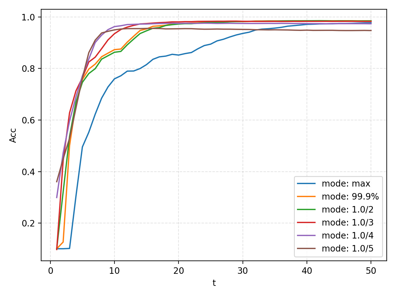
Different normalization modes trade off early-timestep convergence against final accuracy. Choose based on latency and accuracy requirements.

Conversion recipe comparison

Besides the basic RateCodingRecipe, SpikingJelly also provides LocalThresholdBalancingRecipe for estimating local thresholds during conversion. This recipe follows the local-threshold-balancing method [3]. The following comparison uses the ANN, legacy scalar-threshold RobustNorm, and the LTB recipe. The runnable entrypoint is still spikingjelly.activation_based.ann2snn.examples.cnn_mnist:

python -m spikingjelly.activation_based.ann2snn.examples.cnn_mnist \
  --time-steps 32 \
  --output /tmp/ann2snn_mnist_t32.json

The table below is generated by this command. RobustNorm uses RateCodingRecipe(dataloader=..., mode="99.9%"). LTB uses LocalThresholdBalancingRecipe(dataloader=..., time_steps=32, mode="99.9%"). This MNIST run uses all 60000 training samples for calibration and evaluates on the full 10000-image test set:

MNIST CNN conversion results

Method	Calibration samples	Test samples	Timesteps	Top-1 (%)
ANN		10000		98.70
RobustNorm (legacy, scalar threshold)	60000	10000	32	98.35
LocalThresholdBalancingRecipe	60000	10000	32	98.53

ResNet-18 conversion

The ImageNet ResNet-18 example demonstrates the same recipes on a larger classification model. It uses torchvision ResNet18_Weights.IMAGENET1K_V1 and the corresponding preprocessing. The calibration set is a deterministic 50000-image subset from ImageNet train, and the evaluation set is the full 50000-image ImageNet validation set. The command assumes that /path/to/imagenet contains train/ and val/. If your dataset is nested under an additional directory such as ILSVRC2012/, point --data-root to the directory that directly contains train/ and val/.

备注

LocalThresholdBalancingRecipe in SpikingJelly is an engineering implementation of the main local-threshold-balancing idea within the current ANN2SNN recipe framework. It is not a full reproduction of the original LTB paper pipeline [3]. Some paper-specific engineering details and evaluation settings are intentionally not included. Therefore, the accuracy below should be interpreted as the result of this SpikingJelly recipe implementation, not as the official accuracy of the LTB paper or a directly comparable reproduction.

Run the example as follows:

CUDA_VISIBLE_DEVICES=0 python -m spikingjelly.activation_based.ann2snn.examples.imagenet_resnet18_ltb \
  --data-root /path/to/imagenet \
  --calib-samples 50000 \
  --batch-size 128 \
  --num-workers 8 \
  --device cuda:0 \
  --time-steps 32 \
  --recipes ann robust_legacy ltb \
  --delay-start auto \
  --output /tmp/ann2snn_imagenet_t32_delayauto_calib50k_tutorial.json

The robust_legacy recipe name denotes the legacy scalar-threshold RateCodingRecipe without channel_wise or half_threshold. --delay-start auto estimates the delayed-readout start timestep before evaluation and skips the early transient SNN timesteps. It only changes the readout window and does not change the converted neuron dynamics. In the full LTB run below, the estimated delay_start is 27; the exact value can vary with the model, calibration data, and implementation details.

ImageNet ResNet-18 conversion results

Method	Calibration samples	Validation samples	Timesteps	Top-1 (%)	Top-5 (%)
ANN		50000		69.756	89.074
RobustNorm (legacy, scalar threshold)	50000	50000	32	12.462	28.662
LocalThresholdBalancingRecipe	50000	50000	32	65.472	86.636

Scalar-threshold robust normalization without per-channel normalization achieves only 12.462% Top-1 on this deeper ImageNet CNN. The LTB recipe raises it to 65.472% Top-1.

[1] (1,2,3,4,5,6,7)

Rueckauer B, Lungu I-A, Hu Y, Pfeiffer M and Liu S-C (2017) Conversion of Continuous-Valued Deep Networks to Efficient Event-Driven Networks for Image Classification. Front. Neurosci. 11:682.

[2]

Diehl, Peter U. , et al. Fast classifying, high-accuracy spiking deep networks through weight and threshold balancing. Neural Networks (IJCNN), 2015 International Joint Conference on IEEE, 2015.

[3] (1,2)

Bu T, Li M, Yu Z. Inference-Scale Complexity in ANN-SNN Conversion for High-Performance and Low-Power Applications. arXiv:2409.03368, 2024. Accepted by CVPR 2025.

Additional references:

• Rueckauer, B., Lungu, I. A., Hu, Y., & Pfeiffer, M. (2016). Theory and tools for the conversion of analog to spiking convolutional neural networks. arXiv preprint arXiv:1612.04052.

• Sengupta, A., Ye, Y., Wang, R., Liu, C., & Roy, K. (2019). Going deeper in spiking neural networks: Vgg and residual architectures. Frontiers in neuroscience, 13, 95.