Distributed SNN Training and Inference

Authors: Yifan Huang (AllenYolk), Wei Fang (fangwei123456)

中文版： SNN 分布式训练与推理

This page covers high-level training, evaluation, and offline inference APIs, custom model and loop integration, and throughput and memory results from four RTX 4090 GPUs. Vision and LLM use different precision entry points; see Training and Inference Precision.

API design rationale

The API separates vision and llm workloads. Spiking CNNs are organized around channels and feature maps, whereas LLMs are organized around tokens, attention, and context parallelism. Sharing one model description would add branches rather than simplify either path. The common vocabulary remains small: ModelConfig describes a model, ModelBuilder connects its implementation, TrainingConfig and EvaluationConfig describe training and labeled evaluation, and prediction or generation configs describe unlabeled output.

Parallel execution comes from the native runtime whenever possible. PyTorch provides DP, FSDP2, device meshes, and Vision pipelines. Megatron Core provides LLM TP, PP, CP, the distributed optimizer, and sharded checkpoints. SpikingJelly adds SNN temporal layout, state reset, channel-sharded layers, and memopt. An LLM builder returns MCore's model_provider / forward_step callbacks; a Vision builder returns pipeline stages, FSDP2 roots, and boundary shapes. High-level entry points own lifecycle management, while custom workloads can compose the low-level pieces directly.

High-level APIs

Vision models

spikingjelly.activation_based.distributed.vision provides image classification training with PyTorch DDP, FSDP2, tensor parallelism, and pipeline parallelism. vision.TrainingConfig describes the job and vision.train_classification executes it:

from pathlib import Path

from spikingjelly.activation_based.distributed import vision
from spikingjelly.activation_based.model.sew_resnet import SEWResNet34Config
from spikingjelly.activation_based.precision import PrecisionConfig

config = vision.TrainingConfig(
    model=SEWResNet34Config(
        time_steps=4, num_classes=1000, step_mode="m"
    ),
    dataset_builder=(
        "spikingjelly.activation_based.distributed.vision."
        "build_imagefolder_datasets"
    ),
    dataset_kwargs={"root": Path("/datasets/imagenet")},
    input_layout="NCHW",
    batch_size=32,
    loss_function="torch.nn.functional.cross_entropy",
    loss_kwargs={"label_smoothing": 0.1},
    tensor_parallel_size=2,
    data_parallel="fsdp2",
    precision=PrecisionConfig(mode="bf16"),
    memopt_level=1,
    memopt_checkpoint_budget="balanced",
)
metrics = vision.train_classification(config)

PrecisionConfig is prepared before DDP/FSDP wrapping and optimizer creation. Experimental Transformer Engine FP8 and Triton-neuron mixed precision currently require DDP with TP=PP=1. MCore LLM precision is independent and remains configured through its native transformer and optimizer configuration. See Training and Inference Precision for configuration ownership, standalone usage, and measured FP8 crossover points.

batch_size is the batch size on each DP rank. The global batch is batch_size * DP and does not include TP, PP, or SNN time steps. tensor_parallel_size and pipeline_parallel_size select TP and PP; the remaining ranks become DP replicas. Model-owned distributed recipes are imported from model.sew_resnet and model.spikformer rather than distributed.vision. The included examples are SEWResNet34Config, SpikformerConfig, and SpikformerCIFAR10Config. The CIFAR-10 variant fixes the official 32×32 input, 4×4 patch stem, 384 channels, 12 attention heads, and 4 transformer blocks while retaining the same TP, PP, and FSDP2 implementation. mixup_alpha enables serializable batch-level mixup; 0 disables it. Rank zero prints one JSON record after every epoch containing the optimizer step, train loss, validation loss, and validation accuracy. The returned metrics dictionary contains the final values and throughput statistics.

input_layout explicitly declares the DataLoader batch layout. "NCHW" accepts static [N, C, H, W] images; single-step calls the model T times with the same batch, while multi-step constructs contiguous [T, N, C, H, W] input. "NTCHW" accepts default-collated [N, T, C, H, W] frames from datasets such as CIFAR10-DVS and DVS Gesture, validates T, and converts them to time-first layout. Tensor rank is never used to infer the declared layout.

Before parallel wrapping, the entry point calls functional.set_step_mode and resets the model with functional.reset_net after each complete time window. Single-step currently does not support PP, memopt, or the Triton neuron backend. The built-in SEW-ResNet34 supports both modes. Spikformer's architecture and attention are intrinsically multi-step and are not wrapped to simulate a single-step interface. Single-step DDP disables per-forward buffer broadcasts so repeated calls do not modify BatchNorm buffers needed by backward. It instead broadcasts buffers once before each complete T window, keeping replicas synchronized without mutating a saved buffer between single-step forwards.

loss_function is the full import path of a callable receiving reduced [N, C] logits and class targets. It must return the batch-mean scalar used for backward and loss reporting. loss_kwargs supplies keyword arguments to each call. The same function is used by non-pipeline and pipeline training and validation; top-1 accuracy remains the fixed classification metric.

The repository's synthetic-data entry point can verify the installation and parallel configuration directly:

torchrun --standalone --nproc-per-node=4 benchmark/vision_distributed.py \
    --model sew-resnet34 \
    --data-parallel fsdp2 \
    --tensor-parallel-size 2 \
    --precision bf16 \
    --max-steps 10

Custom models use vision.ModelConfig and vision.ModelBuilder. build returns the model for the current rank, FSDP2 shard roots, and PP input/output shapes. See spikingjelly.activation_based.distributed.vision.ModelBuilder for the complete signature.

LLMs

spikingjelly.activation_based.distributed.llm provides SNN language-model training on Megatron Core. It requires Python 3.12 or newer. Install the optional dependency first:

uv pip install --editable ".[megatron]"

llm.TrainingConfig combines:

• an llm.ModelConfig containing the MCore TransformerConfig, vocabulary, context, and SNN time steps;

• an MCore OptimizerConfig;

• the dataset builder, micro/global batch, training progress, evaluation, and checkpoint settings;

• optional SpikingJelly memopt.

When no topology is specified, llm.plan_training selects TP, PP, CP, and recomputation from the GPU count, memory budget, and objective. For a known topology, set TransformerConfig directly. The complete SpikeLM model, optimizer, and dataset configuration lives in benchmark/snn_llm/cli.py:

torchrun --standalone --nproc-per-node=4 \
    benchmark/snn_llm/train_spikelm.py \
    --data /datasets/tokens \
    --output checkpoints/spikelm \
    --train-steps 200 \
    --global-batch-size 128

llm.train currently supports only complete, independent fixed-T windows. The architecture-specific forward_step owns temporal encoding, state isolation, and reduction. Its MCore T*B envelope is not the generic SpikingJelly step_mode="m" interface, so LLM configs intentionally do not expose a step_mode field yet.

Offline distributed inference

Interface roles

Inference interfaces are divided by whether execution belongs to the training lifecycle and whether ground truth is required. Validation and test use the same evaluation computation and differ only in invocation time and dataset, so there are no duplicate validate and test functions.

Vision and LLM inference interface roles

Scenario	Ground truth	Vision	LLM	Output
Validation during training	Required	train_classification evaluates the validation dataset every epoch	train evaluates according to eval_interval / eval_steps	Validation loss/accuracy or LM loss
Post-training evaluation/test	Required	evaluate_classification	MCore evaluate	Aggregate loss, accuracy/perplexity, and performance metrics
Post-training direct prediction/generation	Not required	predict_classification	MCore generate	Per-sample logits or generated tokens; no evaluation metrics
Post-training scheduler-backed offline generation	Not required	—	SGLang open_sglang_engine	Per-request generated tokens; no evaluation metrics

evaluate_classification requires every dataset item to be (image, target). Likewise, llm.evaluate requires input_ids, labels, and an optional loss_mask. Prediction and generation do not read ground truth: Vision ignores targets even if items are (image, target), while LLM generation accepts prompts only. All four roles belong to training or offline workflows. SGLang Engine includes an internal execution scheduler for requests and the KV pool, but the SpikingJelly path includes no HTTP server, router, or other online-serving control plane.

Vision

Vision inference remains native PyTorch. First export a training checkpoint to a TP/PP-independent canonical artifact, then evaluate it under a different DP, FSDP2, TP, or PP topology:

torchrun --standalone --nproc-per-node=4 benchmark/vision_inference.py \
    --artifact artifacts/sew-resnet34.pt \
    --export-checkpoint checkpoints/step_00000010 \
    --model sew-resnet34

torchrun --standalone --nproc-per-node=4 benchmark/vision_inference.py \
    --artifact artifacts/sew-resnet34.pt \
    --model sew-resnet34 \
    --data-parallel replicate \
    --batch-size 32

vision.evaluate_classification returns global loss, accuracy, images/s, and the busiest rank's peak memory. vision.predict_classification computes and returns none of those metrics; it merges rank outputs by dataset index into one HDF5 file containing only index and logits. Classes can be derived with logits.argmax(axis=1). Padding never appears in the final output, so dataset size need not divide DP or batch size.

LLMs

LLMs expose two backends with different roles:

• MCore reuses the training model provider and sharded checkpoint. It serves validation, loss/perplexity evaluation, and synchronous generation with direct tensor-batch semantics. llm.evaluate(EvaluationConfig(...)) runs complete DP/TP/PP/CP loss and perplexity evaluation. llm.generate(MCoreGenerationConfig(...), input_ids) adds DP prompt sharding to TP/PP static-KV-cache generation. MCore cached generation requires CP=1.

• SGLang handles scheduler-backed, high-throughput post-training offline generation. open_sglang_engine() manages the native Engine lifecycle; sampling, variable-length token IDs, asynchronous generation, and streaming use the native Engine interface. It starts no HTTP server or router.

Choosing an LLM inference backend

Requirement	Backend
Validation, loss/perplexity, or direct training-checkpoint restore	MCore
Explicit local/global batch, pipeline microbatch, and CUDA OOM semantics	MCore
Large prompt corpus, continuous batching, and KV-cache scheduling	SGLang
HTTP/router, multi-tenancy, or SLA serving	Out of scope

MCore evaluation and SGLang generation answer different questions and cannot be compared with one shared batch, memory, or throughput protocol.

SGLang 0.5.17 uses its own PyTorch and Transformers stack. Create a separate environment:

uv venv --python 3.12 .venv-sglang
source .venv-sglang/bin/activate
uv pip install --editable ".[sglang]"

llm.export_sglang_artifact owns distributed checkpoint loading, per-stage sharded writes, indexing, failure synchronization, and atomic publication. A model-owned stage_tensors callback supplies weight names and transformations, while artifact_config supplies the SGLang/Hugging Face configuration. Run export with torchrun using the checkpoint's TP x PP x CP topology; no GPU gathers the complete model, and the resulting artifact may use another TP/PP/DP topology at inference.

The repository's SpikeLM and Qwen2 recipes and external runtime models live in benchmark/snn_llm and demonstrate this seam; they are not wheel-installed model support. Their adapters retain hidden state as [token, T, hidden] and fold T into the head dimension only at the RadixAttention/KV-cache seam. A custom model must provide both its export callback and an importable SGLang external model package.

The current runtime supports single-node NVIDIA BF16 TP, PP, and DP. Prefill CP and DCP are unsupported. CUDA Graph is disabled because the temporal adapters do not yet provide the attention metadata required by SGLang 0.5.17 graph capture. The adapters use SGLang's native layer staging and PPProxyTensors protocol.

from pathlib import Path

from spikingjelly.activation_based.distributed import llm

def main():
    config = llm.SGLangEngineConfig(
        artifact=Path("artifacts/qwen2-snn"),
        external_model_package="benchmark.snn_llm.sglang_models",
        tensor_parallel_size=2,
    )
    with llm.open_sglang_engine(config) as engine:
        outputs = engine.generate(
            input_ids=[[1, 2, 3], [1, 2, 3, 4, 5]],
            sampling_params={"temperature": 0, "max_new_tokens": 32},
        )
    print(outputs)

if __name__ == "__main__":
    main()

benchmark/snn_llm/sglang_benchmark.py provides reproducible offline Engine measurements. The experimental protocol, throughput/latency metrics, and results are kept together in the SGLang subsection under “Measured results.”

Low-level APIs

Custom vision models

vision.ModelBuilder.build constructs the current PP stage, applies model parallelism, and returns the FSDP2 shard roots. See SEWResNet34Builder and SpikformerBuilder for working implementations.

A minimal declaration has this form. It defines no model-specific checkpoint boundaries, so it rejects a nonzero memopt_level. A real implementation should apply memopt before returning, as the built-in builders do.

from dataclasses import dataclass
from typing import ClassVar

from spikingjelly.activation_based.distributed import vision

@dataclass(frozen=True)
class MyModelConfig(vision.ModelConfig):
    builder: ClassVar[str] = "my_package.model.MyModelBuilder"
    width: int = 128

class MyModelBuilder(vision.ModelBuilder):
    def build(
        self,
        *,
        process_group,
        memopt_process_group,
        pipeline_rank,
        pipeline_size,
        pipeline_microbatches,
        device,
        micro_batch_size,
        memopt_level,
        memopt_compress_inputs,
        memopt_checkpoint_budget,
    ):
        if pipeline_size != 1:
            raise ValueError("MyModelBuilder does not define PP stages.")
        if memopt_level:
            raise ValueError("MyModelBuilder does not define memopt rules.")
        model = build_my_model(self.config)
        model = parallelize_my_model(model, process_group)
        model.to(device)
        return model, ("blocks",), None, None

The model author supplies parallelize_my_model. This example replaces model layers with public components from spikingjelly.activation_based.distributed.tensor_parallel:

from spikingjelly.activation_based.distributed.tensor_parallel import (
    ChannelShardBatchNorm2d,
    ChannelShardConv2d,
)

def parallelize_my_model(model, process_group):
    block = model.block
    block.conv1 = ChannelShardConv2d(block.conv1, process_group, "colwise")
    block.bn1 = ChannelShardBatchNorm2d(block.bn1, process_group)
    block.conv2 = ChannelShardConv2d(block.conv2, process_group, "rowwise")
    return model

The neuron consumes the local-channel tensor produced by the colwise layer directly; no wrapper is required. The model author only needs to ensure that the following rowwise layer consumes that local tensor.

Custom training loops

When the predefined train does not fit the task, compose the PyTorch distributed interfaces with the SpikingJelly components above. The following omits the task-specific build_my_model, dataset, and hyperparameters and shows only the assembly order:

import os

import torch
import torch.distributed as dist
from torch.distributed.device_mesh import init_device_mesh
from torch.nn.parallel import DistributedDataParallel
from torch.utils.data import DataLoader, DistributedSampler

from spikingjelly.activation_based import functional

local_rank = int(os.environ["LOCAL_RANK"])
torch.cuda.set_device(local_rank)
dist.init_process_group("nccl", device_id=torch.device("cuda", local_rank))

mesh = init_device_mesh(
    "cuda", (dp_size, tp_size), mesh_dim_names=("dp", "tp")
)
dp_group = mesh["dp"].get_group()
tp_group = mesh["tp"].get_group()

model = build_my_model()
model = parallelize_my_model(model, tp_group).cuda(local_rank)
functional.set_step_mode(model, step_mode)
model = DistributedDataParallel(
    model, device_ids=[local_rank], process_group=dp_group
)
optimizer = torch.optim.AdamW(model.parameters(), lr=1e-3)

sampler = DistributedSampler(
    dataset,
    num_replicas=dp_size,
    rank=mesh.get_local_rank("dp"),
    shuffle=True,
)
loader = DataLoader(dataset, batch_size=local_batch_size, sampler=sampler)

for epoch in range(epochs):
    sampler.set_epoch(epoch)
    for images, labels in loader:
        images = images.cuda(local_rank, non_blocking=True)
        labels = labels.cuda(local_rank, non_blocking=True)
        sequence = (
            images.unsqueeze(0)
            .expand(time_steps, *images.shape)
            .contiguous()
        )

        optimizer.zero_grad(set_to_none=True)
        if step_mode == "s":
            logits = torch.stack([model(x_t) for x_t in sequence]).mean(0)
        else:
            logits = model(sequence).mean(0)
        loss = torch.nn.functional.cross_entropy(logits, labels)
        loss.backward()
        optimizer.step()
        functional.reset_net(model)

Validation, mixed precision, scheduling, metric reduction, and checkpoints are task-specific. The following calling contracts are required:

• world size must be divisible by the selected model-parallel size;

• data is sharded only over DP, and ranks in one TP group receive the same batch;

• create the optimizer after model parallelism and DDP/FSDP2 wrapping;

• reset SNN state after every independent batch or pipeline microbatch;

• global batch excludes TP, PP, CP, and SNN time steps.

Custom LLMs

An LLM subclasses llm.ModelConfig and points its builder class variable to an llm.ModelBuilder. The builder's build method returns the MCore model_provider and forward_step callbacks:

from dataclasses import dataclass
from typing import ClassVar

from spikingjelly.activation_based.distributed import llm

@dataclass(frozen=True, kw_only=True)
class MyModelConfig(llm.ModelConfig):
    builder: ClassVar[str] = "my_package.model.MyModelBuilder"

class MyModelBuilder(llm.ModelBuilder):
    def build(
        self,
        *,
        memopt_level: int = 0,
        memopt_checkpoint_budget: str = "memory",
        resume: bool,
    ):
        return model_provider, forward_step

model_provider builds the current PP stage. forward_step reads one microbatch from the data iterator, invokes the model, and returns the MCore loss callback. These callbacks can be passed to llm.train or used in a custom MCore training loop. Complete SpikeLM and Qwen2 implementations are available in benchmark/snn_llm/spikelm.py and benchmark/snn_llm/qwen2.py.

The SNN temporal layout is [T, B, S, H] -> [S, T*B, H]. T is folded only into the MCore batch dimension. It is not folded into the token dimension and does not contribute to global batch size.

Measured results

The Vision and MCore results below were measured on one 4 x RTX 4090 24-GiB host without NVLink or CUDA peer access. Its software stack used PyTorch 2.8.0, Megatron Core 0.18.2, and Triton 3.4.0. SGLang used separate rentals with the same GPU/interconnect class and its own pinned runtime, described in that subsection. Treat these as relative references for PCIe multi-GPU hosts; NVLink systems need separate measurements.

Vision training benchmarks

The Vision benchmarks fixed BF16, T=4, 128 x 128 inputs, and 1000 classes. The plots retain only one GPU, DP4, FSDP4, TP4, and PP4. Each curve labels its largest successful global batch size (G). For one GPU, TP4, and PP4, global batch equals per-rank batch; for DP4 and FSDP4 it is four times larger.

All topologies at a fixed global batch

The table gives the complete topology comparison at G=32. Each configuration started in a fresh process, warmed up for 10 optimizer steps, measured 50 steps, and was repeated independently three times. Values are the three-run medians. Throughput covers the whole job; memory is the highest CUDA peak allocated memory among all ranks.

Vision results across all topologies at fixed G=32

Topology	GPUs	SEW-ResNet34 images/s	SEW-ResNet34 GiB/GPU	Spikformer-S images/s	Spikformer-S GiB/GPU
One GPU	1	269.0	1.67	270.1	3.15
DP2	2	261.8	1.15	264.3	1.73
FSDP2	2	146.9	0.86	172.6	1.59
TP2	2	257.6	1.30	262.6	2.03
PP2	2	83.9	1.01	85.9	2.20
DP4	4	259.9	0.82	258.8	1.00
FSDP4	4	145.7	0.45	169.4	0.81
TP4	4	240.3	1.10	246.9	1.45
PP4	4	122.2	0.75	148.5	1.71
TP2 + DP2	4	244.8	0.82	251.3	1.10
TP2 + FSDP2	4	143.3	0.65	166.7	1.01
PP2 + DP2	4	150.9	0.53	146.3	1.18
PP2 + FSDP2	4	74.4	0.52	86.2	1.13
TP2 + PP2	4	81.9	0.86	82.0	1.45

At the same G=32, multiple GPUs primarily reduce per-GPU memory. As compute per GPU shrinks, PCIe communication, synchronization, and pipeline bubbles dominate more easily. The capacity curves below instead increase global batch and compare each strategy's throughput-memory frontier.

Batch size was increased by powers of two until the first candidate that could not complete. SEW-ResNet34 succeeded through per-rank batch 256 on one GPU, DP4, and FSDP4, and through 512 on TP4 and PP4. Each configuration started in a fresh process, warmed up for 10 optimizer steps, and measured 40 steps. Spikformer-S succeeded through per-rank batch 128 on one GPU, DP4, and FSDP4, and through 256 on TP4 and PP4, with 5 warmup and 25 measured steps. Every successful point was repeated independently three times; the plots show the median and three-run range. Timing includes H2D, forward, backward, communication, and the optimizer, but excludes initialization, DataLoader work, validation, and checkpoints.

The vertical axis is aggregate job throughput: global batch divided by the slowest rank's measured time. The horizontal axis is the highest CUDA peak allocated memory among all ranks. Both axes are logarithmic; failed candidates are omitted.

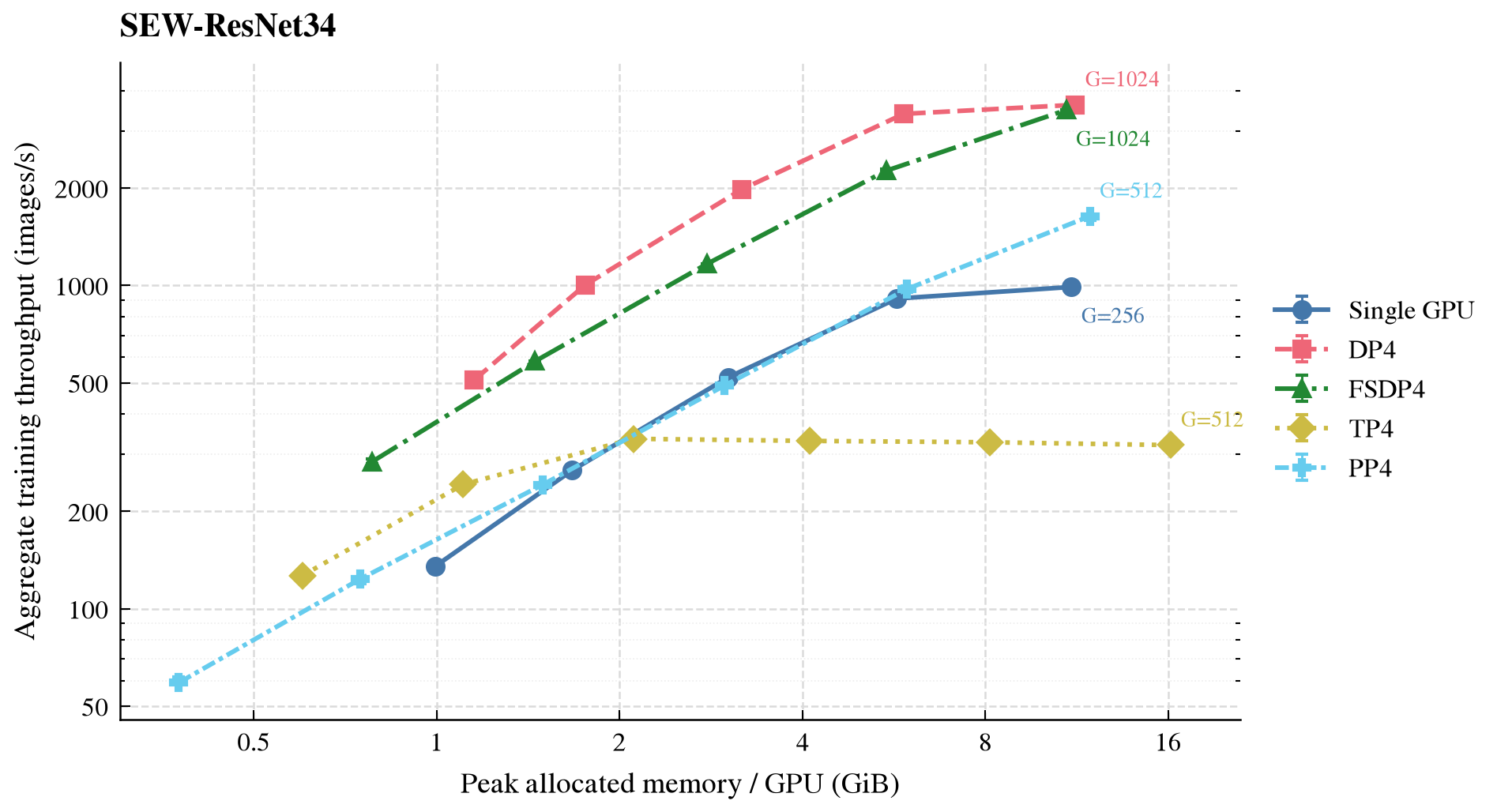
SEW-ResNet34 aggregate training throughput versus the busiest GPU's peak allocated memory.

Spikformer-S aggregate training throughput versus the busiest GPU's peak allocated memory.

SEW-ResNet34 DP4 reached 3616.2 images/s and 11.25 GiB/GPU at G=1024; FSDP4 reached 3482.5 images/s and 10.86 GiB/GPU, while PP4 reached 1636.5 images/s at G=512. The largest successful Spikformer-S points for DP4 and FSDP4 both used G=512 and reached 2503.8 and 2334.6 images/s; PP4 reached 1028.2 images/s at G=256. TP4 plateaued early on both models: increasing batch primarily raised memory, indicating that TP communication dominates on this PCIe host. These numbers describe the throughput-capacity frontier under more total work, not fixed-batch speedup.

Vision capacity search (largest success → first failed candidate)

Model	Topology	Largest successful B/G	First failed B/G	Result
SEW-ResNet34	One GPU	256/256	512/512	CUDA OOM
SEW-ResNet34	DP4	256/1024	512/2048	CUDA OOM
SEW-ResNet34	FSDP4	256/1024	512/2048	CUDA OOM
SEW-ResNet34	TP4	512/512	1024/1024	CUDA OOM
SEW-ResNet34	PP4	512/512	1024/1024	NCCL collective timeout
Spikformer-S	One GPU	128/128	256/256	CUDA OOM
Spikformer-S	DP4	128/512	256/1024	CUDA OOM
Spikformer-S	FSDP4	128/512	256/1024	CUDA OOM
Spikformer-S	TP4	256/256	512/512	NCCL collective timeout
Spikformer-S	PP4	256/256	512/512	NCCL collective timeout

B is the per-rank batch. A collective timeout means that the candidate produced no training metrics; it is neither a slow successful point nor labeled as OOM without an OOM traceback.

LLM training benchmarks

The LLM benchmark used an approximately 1.41B-parameter SpikeLM with 24 layers, hidden size 2048, 16 heads, FFN size 8192, vocabulary 50304, BF16, sequence 128, and T=4. Every capacity-search point below disabled SpikingJelly memopt and gradient accumulation, so global_batch_size = micro_batch_size × data_parallel_size and each optimizer step executes one micro batch on every DP rank.

All topologies at a fixed global batch

The following table is the fixed-work comparison across every tested two-GPU, four-GPU, and hybrid topology: micro batch=1, G=8, 10 warmup optimizer steps, 30 measured steps, and three independent repeats. Values are the three-run medians. One GPU OOMed during distributed-optimizer initialization, so DP2 is the relative-throughput baseline. Holding G=8 across different DP sizes required 8 / DP accumulation steps in this fixed-work experiment: four for DP2, two for DP4, and eight for each DP1 topology. It is a different protocol from the no-accumulation capacity search below.

1.41B SpikeLM results across all topologies at fixed G=8

Topology	GPUs	Semantic tokens/s	GiB/GPU	Relative to DP2
DP2	2	746.3	17.35	1.00x
TP2	2	679.9	12.86	0.91x
PP2	2	1008.3	13.15	1.35x
CP2	2	417.7	16.56	0.56x
DP4	4	585.6	13.40	0.78x
TP4	4	673.1	6.65	0.90x
PP4	4	1379.9	8.09	1.85x
CP4	4	289.5	12.34	0.39x
TP2 + DP2	4	817.1	8.91	1.09x
PP2 + DP2	4	997.9	9.20	1.34x
CP2 + DP2	4	446.0	12.61	0.60x
TP2 + PP2	4	989.1	6.81	1.33x
TP2 + CP2	4	427.2	8.39	0.57x
PP2 + CP2	4	612.6	8.44	0.82x

At fixed G=8, PP4 has the highest aggregate throughput, while TP4 and TP2 + PP2 have the lowest per-GPU peak memory. CP cannot amortize its communication at sequence length 128. This table compares topologies directly; the following no-accumulation experiment compares their batch-capacity and throughput limits.

The plot retains DP2, DP4, TP4, PP4, and CP4. DP2 succeeds only through micro batch 1 (G=2), DP4 through micro batch 4 (G=16), and TP4, PP4, and CP4 through micro batch 16 (G=16). Each configuration started in a fresh process, warmed up for 5 steps, measured 15 steps, and was repeated independently three times. One GPU OOMed during distributed-optimizer initialization and is omitted. The LLM path uses MCore DDP and its distributed optimizer rather than PyTorch FSDP2.

1.41B SpikeLM training throughput versus peak memory per GPU, without gradient accumulation or memopt.

PP4 at G=16 reached 2997.4 semantic tokens/s and 14.85 GiB/GPU, the highest throughput in this set; it is already close to the 2897.0 tokens/s measured at G=8. TP4 reached 1684.4 tokens/s and 16.47 GiB/GPU at G=16 and likewise flattened noticeably after G=4. DP4's largest successful point remains G=16 at 1284.3 tokens/s and 17.55 GiB/GPU. CP4 reached 865.5 tokens/s and 16.52 GiB/GPU after scaling to G=16, but remained below TP4 and PP4. DP2 retains only G=2 at 303.0 tokens/s and 17.35 GiB/GPU.

LLM capacity search (largest success → first failed candidate)

Topology	Largest successful micro/G	First failed micro/G	Result
DP2	1/2	2/4	CUDA OOM
DP4	4/16	8/32	CUDA OOM
TP4	16/16	32/32	CUDA OOM
PP4	16/16	32/32	stalled, no training metrics
CP4	16/16	32/32	stalled, no training metrics

The PP4 and CP4 micro=32 candidates remained in fixed rank-wait states and were terminated as stalled; they are not throughput points.

Points on different curves can have different global batches, so this plot shows the throughput-capacity frontier rather than fixed-batch speedup. Complete medians, three-run ranges, and batch configurations are available in the summary CSV.

Functional tests also covered BF16 TP4, PP4, TP2 x PP2, CP4, TP2 x CP2, and PP2 x CP2, plus FP8 TP4, PP4, and CP4. Every case produced finite loss and gradients and nonzero gradients in the SNN modules. Under a 7-GiB memory budget, the planner selected TP4, SpikingJelly memopt, and MCore selective core_attn recomputation. The 6.28 GiB figure is the static planning input; forcing this plan for two training steps reached about 7.26 GiB/GPU in practice. A TP2 x PP2 sharded model/optimizer checkpoint also resumed successfully from step 1 to step 2.

Distributed inference benchmarks

Common environment

The inference benchmark used the same single-host 4 x RTX 4090 24-GiB environment as training. nvidia-smi topo -m reports SYS from GPU0 to every other GPU and NODE among GPUs 1--3, with no NV# link. nvidia-smi topo -p2p r/w returns CNS for every GPU pair. The host therefore has neither NVLink nor a usable CUDA peer read/write path; NCCL traffic traverses PCIe/CPU interconnects. The Vision/MCore stack matches training: PyTorch 2.8.0, Megatron Core 0.18.2, and Triton 3.4.0.

Vision evaluation

The historical curves below used BF16, T=4, 1000 classes, and a cached all-zero 224 x 224 image. Current runs instead pass --cifar10-data or --data for a fixed real-image subset; the seeded-random default is for smoke tests. Results from the two protocols remain separate.

Each throughput point starts in a fresh process with four DataLoader workers, five warmup batches, ten measured batches, and three independent repeats. Timing includes H2D, forward, communication, and metric reduction, but excludes DataLoader work, artifact loading, and initialization. The plots show every three-run completion with its median and range.

L denotes local batch per DP replica and G = L × DP denotes global batch; TP, PP, CP, and T do not multiply G. For PP, K is the number of pipeline microbatches and each chunk has size L / K. The non-PP SEW-ResNet34 grid is 16, 32, 64, 96, 128, 192, 256, 384, 512, 768, 1024; Spikformer-S stops between 384 and 1024 according to OOM. PP4 fixes K=4 and extends SEW-ResNet34 to L=3072 and Spikformer-S to L=1536. Capacity searches try 2x and then 1.5x from each successful point until CUDA OOM.

Inference PP uses a forward-only streaming schedule and synchronizes the pipeline group before returning each high-level batch. SEW downsampling blocks precede stage boundaries; Spikformer blocks are split 0/2/2/2. pipeline_microbatches defaults to one, while the Vision and MCore PP points here fix it at four, so chunk size grows as L/4. The CSV records L, G, K, chunk size, and failed candidates.

Complete SEW-ResNet34 batch sweeps with PP K fixed at 4.

Complete Spikformer-S batch sweeps with PP K fixed at 4.

At per-rank batch 128, SEW-ResNet34 reaches 845.7, 3368.9, 3109.3, 548.3, and 1320.9 images/s on one GPU, DP4, FSDP4, TP4, and PP4. Spikformer-S reaches 516.6, 2060.4, 2000.2, 412.2, and 1088.5 images/s. DP/FSDP approach linear four-GPU throughput. PP reaches 1.56x and 2.11x single-GPU throughput. With K fixed, PP peaks at a medium batch and then moves smoothly into its capacity tail as per-chunk samples and memory continue to grow.

Pure TP4 remains below one GPU but is now stable; this is a model compute-to-communication limit rather than scheduler variance. SEW executes 16 rowwise all-reduces totaling about 1.41 GB per batch, while Spikformer executes 12 totaling about 0.92 GB. Two TP2 replicas on four GPUs reach 1226.1 and 858.6 images/s, so practical deployments use TP to fit the model and DP to scale throughput.

Vision inference capacity boundaries

Model	Topology	Largest three-run L/G	First failure and final capacity evidence
SEW-ResNet34	One GPU	512/512	768/768: sustained multi-batch CUDA OOM
SEW-ResNet34	DP4	512/2048	768/3072: sustained multi-batch CUDA OOM
SEW-ResNet34	FSDP4	512/2048	768/3072: sustained multi-batch CUDA OOM
SEW-ResNet34	TP4	512/512	768/768: sustained multi-batch CUDA OOM
SEW-ResNet34	PP4	3072/3072	4096/4096: CUDA OOM
Spikformer-S	One GPU	256/256	384/384: CUDA OOM
Spikformer-S	DP4	384/1536	512/2048: CUDA OOM
Spikformer-S	FSDP4	256/1024	384/1536: CUDA OOM
Spikformer-S	TP4	512/512	768/768: CUDA OOM
Spikformer-S	PP4	1536/1536	2048/2048: CUDA OOM

Vision correctness tests also covered FSDP2, PP2, and exporting a TP2 x PP2 training checkpoint before restoring it on four single-GPU replicas (DP4). Validation loss was 2.310132205 before export and 2.310132384 after restore.

MCore loss/perplexity evaluation

MCore loss/perplexity evaluation uses Qwen2.5-0.5B QCFS, BF16, T=2, and sequence length 16. It compares one GPU, DP4, TP2, PP2, and PP4. With 14 attention heads, TP2 is the only valid pure-TP option above one. The one-GPU and DP4 runs use a fixed 128-sample dataset; TP2/PP2/PP4 set sample count to G so padding does not affect throughput.

Each point restores the same sharded checkpoint in a fresh process, warms up five schedules, measures a complete schedule, and repeats three times. Timing includes H2D, model execution, communication, and metric reduction; initialization, dataset indexing, and collation are excluded. Runs set NCCL_P2P_DISABLE=1, NCCL_IB_DISABLE=1, and PYTORCH_CUDA_ALLOC_CONF=expandable_segments:True.

Here L equals micro_batch_size × pipeline_microbatches. Non-PP points use K=1 and PP2/PP4 fix K=4, so chunk size grows as L/4. The grid is 16, 32, 64, 96, 128, 192, 256, 384, 512, 768, 1024, followed by the 2x/1.5x capacity search. The PP4 L=3072 debug probe uses one warmup and serves only as capacity evidence.

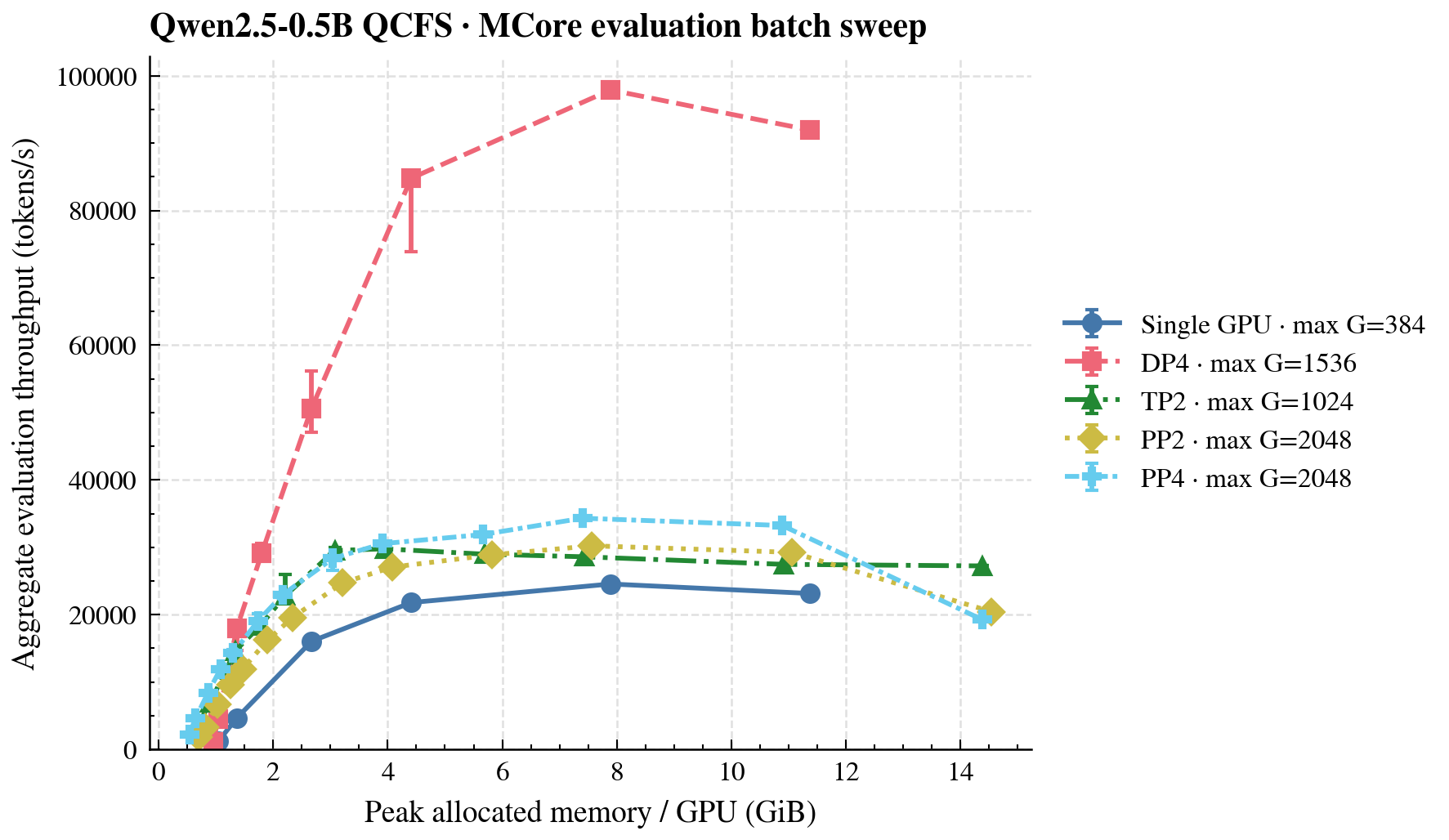
MCore evaluation: aggregate semantic-token throughput versus peak memory per GPU.

At small-batch L=16, one GPU, TP2, PP2, and PP4 reach 4636.2, 3611.2, 1823.5, and 2203.6 semantic tokens/s. With K fixed at 4, each PP chunk contains only four samples, so kernel and schedule overheads are not yet amortized. By L=384, one GPU, TP2, PP2, and PP4 reach 23145.8, 28975.2, 24707.7, and 28348.2 tokens/s; all three model-parallel topologies exceed one GPU at the same L.

The best one-GPU, TP2, PP2, and PP4 points reach 24549.7, 29767.5, 30217.9, and 34317.2 tokens/s. The latter three are 1.21x, 1.23x, and 1.40x the best one-GPU throughput. TP2 peaks at L=256 and 3.95 GiB/GPU; PP2 and PP4 peak at L=1024 and 7.57/7.40 GiB/GPU. Both three-run PP curves extend through L=2048 and about 14.5 GiB/GPU. Their capacity-tail drop repeats across all three runs and is the measured cost of growing each chunk to 512 samples. A single debug capacity probe completes PP4 L=3072 at 21.35 GiB/GPU, but the non-debug formal run times out, so that point is excluded from the curve; L=4096 is a confirmed CUDA OOM.

MCore capacity tail (largest completion → first failure)

Topology	Largest L/G	First failed L/G	Status
One GPU	384/384	512/512	CUDA OOM
DP4	384/1536	512/2048	CUDA OOM
TP2	1024/1024	1536/1536	CUDA OOM
PP2	2048/2048	2304/2304	CUDA OOM
PP4	2048/2048	3072/3072	one debug probe completed but the formal run timed out; 4096 CUDA OOM

Complete medians, ranges, memory, and failed statuses are available in the inference-results CSV. The CSV contains only Vision and MCore evaluation results. Regenerate the plots directly from the summary:

python benchmark/plot_distributed_inference.py \
    docs/source/_static/tutorials/distributed/distributed-inference-tradeoff.csv \
    docs/source/_static/tutorials/distributed

SGLang scheduler-backed generation

benchmark/snn_llm/sglang_benchmark.py measures offline Engine request/input/ output throughput, TTFT, TPOT, end-to-end latency, and peak per-GPU memory. Formal points use on-demand 4 x RTX 4090 hosts without NVLink or CUDA peer read/write. The separate environment uses PyTorch 2.11.0, CUDA 13.0, SGLang 0.5.17, BF16, Triton attention, and disabled CUDA Graphs. Each point runs one warmup, flushes the Radix cache before every timed repeat, and reports the median of three repeats. Qwen and SpikeLM use two rentals of the same class; topology and workload comparisons stay within each model.

The Qwen artifact uses Qwen2.5-0.5B weights and deterministic unit QCFS scales. The SpikeLM artifact is deterministically initialized with 32 layers, hidden size 2560, 20 heads, FFN size 10240, vocabulary 50304, and T=4: exactly 2,775,209,216 parameters. Both are system measurements, not claims about post-training model quality.

Left: one GPU and PP4 output throughput for SpikeLM-2.78B at 32/64 requests; middle: one-GPU and DP4 Qwen2.5-0.5B output throughput; right: one-GPU input/output throughput with shared-prefix reuse.

PP is not an unconditional speedup. At 32 requests with 64 input and 64 output tokens, one-GPU and PP4 SpikeLM-2.78B reach 1074.8 and 786.9 output tokens/s; PP4 is only 0.73x because communication and pipeline bubbles are not amortized. At 64 requests under the same token workload, one GPU reaches 1031.1 tokens/s and PP4 reaches 1416.9 tokens/s, or 1.37x. The p99 TTFT falls from 2430.9 ms to 446.4 ms, while p99 TPOT rises from 33.2 ms to 39.8 ms. On this host, PP4 needs enough concurrency to improve throughput; the result does not imply lower single-request latency.

Qwen2.5-0.5B DP4 uses 32 requests per replica and reaches 5845.5 aggregate output tokens/s, 3.93x the one-GPU 1486.5 tokens/s, with effectively unchanged TPOT. A one-GPU workload with a 2048-token shared prefix raises input throughput 18.3x. The CSV also includes small-model PP2, which remains slower than one GPU. Choose topology for the model size and request concurrency.

The capacity test also exported a 12.6B SpikeLM artifact containing 564 tensors and 25,173,851,048 bytes, then loaded and generated with PP4 without placing the full model on one GPU.

On fixed parity prompts, Qwen2 matched all 32 MCore greedy tokens. SpikeLM matched every first decode token; three of four PP2 prompts matched all eight tokens, while one diverged after the third token under a different BF16 execution order. Near-tied logits do not require identical free-running sequences across backends.

Published medians are available in the SGLang result CSV. Regenerate the figure directly:

python benchmark/plot_sglang_inference.py \
    docs/source/_static/tutorials/distributed/sglang-inference-results.csv \
    docs/source/_static/tutorials/distributed/sglang-inference.png