Training Memory Optimization

Author: Yifan Huang (AllenYolk)

中文版： 训练显存优化

Our new work Towards Lossless Memory-efficient Training of Spiking Neural Networks via Gradient Checkpointing and Spike Compression was published at ICLR 2026. In this work, we propose an automatic memory optimization tool for deep SNN training based on gradient checkpointing and spike compression (source code available on GitHub). With only a few extra lines of code, users can significantly reduce training memory consumption for deep SNNs while keeping accuracy intact and speed slowdown acceptable.

This toolkit has been integrated into the spikingjelly.activation_based.memopt subpackage and can be applied to almost every spikingjelly SNN that operates in multi-step mode. This tutorial shows how to use it.

Method Overview

Memory Footprint Analysis

As shown in Fig. 1, the peak training memory cost of SNNs is far larger than that of ANNs with similar architectures. Intermediate features (light blue bars) account for more than 96% of SNN peak training memory; these features are cached during the forward pass so they can be reused in the backward pass when computing gradients. Therefore, reducing the memory footprint of intermediate features is the key to lowering SNN training memory.

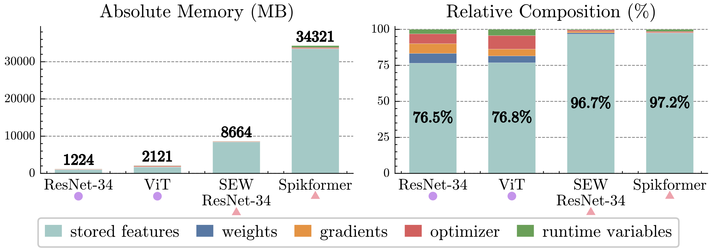
Fig. 1. Memory breakdown at the peak memory moment when training various ANNs and SNNs on ImageNet [1].

If we view a deep SNN as a stack of "weight-norm-neuron" modules (simply called "layers" below), the intermediate features can be divided into two parts:

1. Inputs: usually binary spike tensors. There are exceptions, such as floating-point network inputs or possible non-binary integers in SEW ResNet [2].

2. Internal states: intermediate results inside weights and normalization layers, as well as neuron internal states.

Gradient Checkpointing + Spike Compression

To reduce the memory footprint of internal states, we can apply gradient checkpointing (GC) [3] to every layer. Concretely, during the forward pass of layer \(l\), we only cache its input \(\mathbf{S}^{l-1}\) together with the necessary weights; all internal states are discarded immediately after they are computed. During the backward pass of layer \(l\), we recompute the layer's forward using \(\mathbf{S}^{l-1}\) and the weights to reconstruct internal states before computing gradients. This ensures that at most one layer's internal states live in memory at any time, drastically lowering the peak memory. We call a layer processed this way, which only caches inputs, a GC segment. Compared with a normal layer, a GC segment requires an extra forward pass, so training becomes slower.

Even with layer-wise gradient checkpointing, every layer's input still needs to be cached. Most deep SNN layers take binary spike tensors as their inputs, yet frameworks like spikingjelly store binary tensors using floating-point dtypes (float32, float16, ...). This guarantees computational compatibility but wastes memory. To fix this, we perform lossless spike compression before caching each layer input: the binary floating-point tensor \(\mathbf{S}^{l-1}\) is compressed into a compact representation \(\tilde{\mathbf{S}}^{l-1}\) before caching; during recomputation, we decompress \(\tilde{\mathbf{S}}^{l-1}\) to losslessly recover \(\mathbf{S}^{l-1}\). Experiments show that bit-based compressors (one bit per 0/1 value) offer the best balance between speed and compression ratio, so they serve as the default spike compressor.

Fig. 2(b) illustrates the forward/backward workflow after applying gradient checkpointing plus spike compression. Refer to Algorithm 1 in the original paper for more details [1].

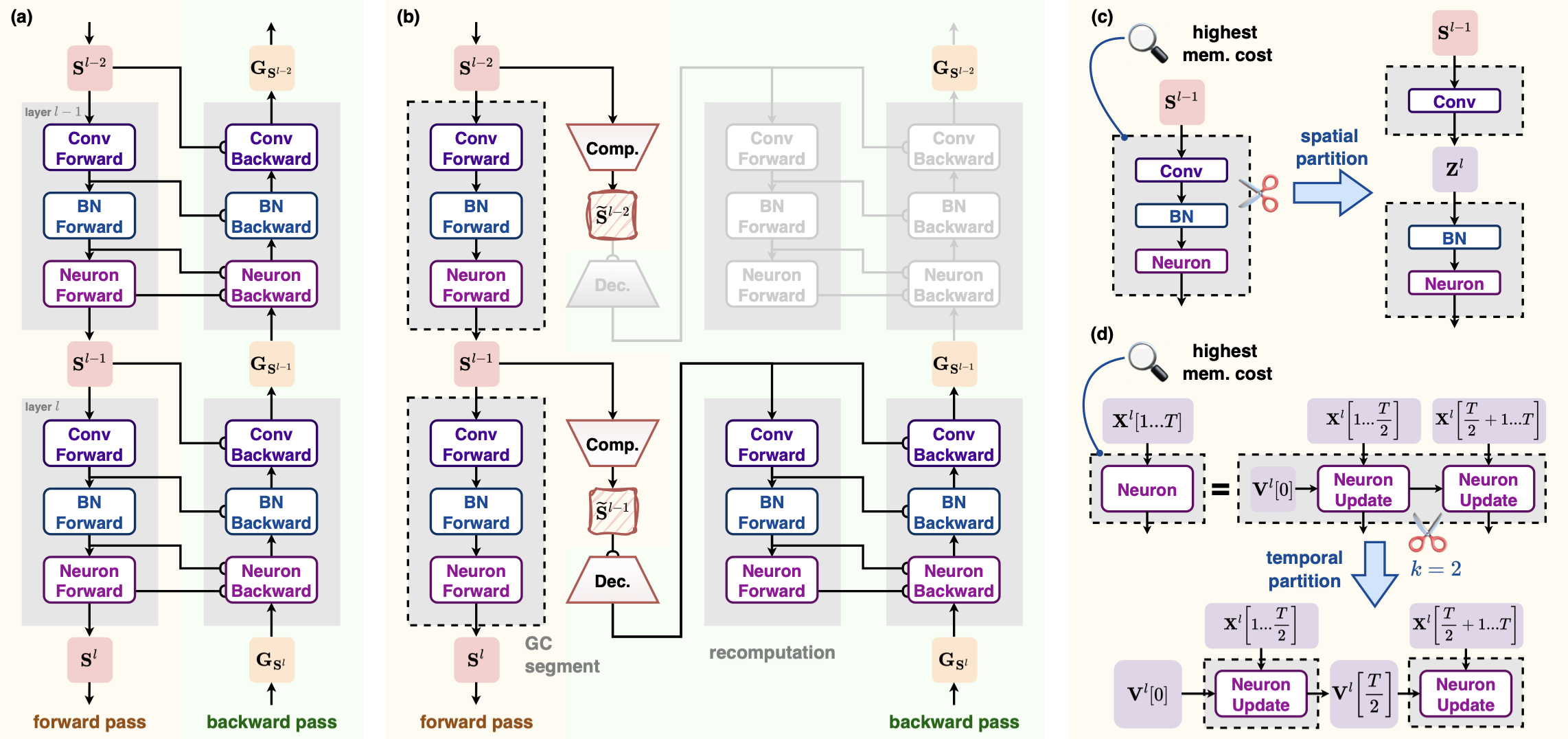
Fig. 2. Method flowchart. Gray rectangles with dashed black borders denote GC segments [1].

Adaptive Adjustment of Checkpoint Structures

After applying per-layer gradient checkpointing and spike compression, the memory evolution within one training iteration looks like the orange curve in Fig. 3. Although the peak is already far lower than vanilla BPTT (blue curve), the global peak is still much higher than the temporary memory usage in other layers. To address this, we design a series of checkpoint splitting strategies. These strategies shrink the size of critical GC segments at the cost of caching more inputs. Additionally, we selectively revert some GC segments back to normal layers to slightly increase temporary memory but speed up training without raising the peak memory. The procedure is:

1. Spatial splitting: Locate the GC segment corresponding to peak memory and split it spatially into two smaller segments. Repeat this until peak memory can no longer be reduced. See Fig. 2(c).

2. Temporal splitting: Locate the peak memory segment and split it along the time dimension into \(k\) smaller segments. Repeat until no further memory reduction. See Fig. 2(d).

3. Greedy restoration: Measure the forward time of every GC segment and sort them in descending order. Try reverting each segment back to a normal layer. If peak memory does not increase after a restoration, keep it; otherwise undo the change.

See Algorithm 2 in the original paper for more details [1].

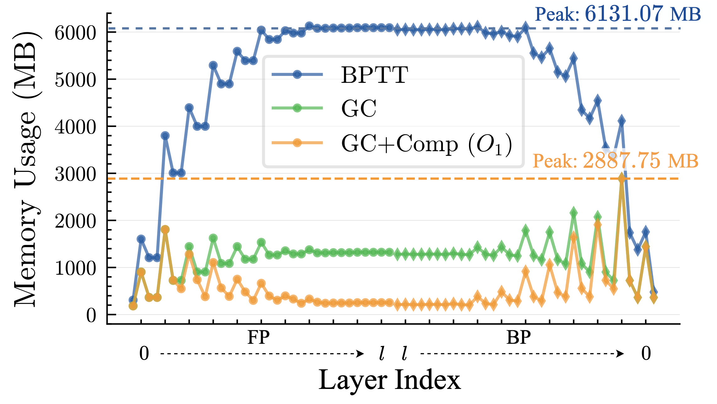
Fig. 3. Memory usage during one training iteration of Spiking VGG on CIFAR10-DVS [1].

备注

Spatial splitting is always tried before temporal splitting. That is, temporal splitting is only a supplementary strategy. That's because temporal splitting is not compatible with temporal parallelism, and it prevents kernel fusion across time steps (a kernel that originally fused \(T\) steps must turn into \(k\) kernels that each handles \(T/k\) steps), which slows things down.

Usage Guide

Implementation Overview

This framework relies on two classes to represent GC segments:

• GCContainer: a subclass of nn.Sequential that contains a sequence of nn.Module members and overrides forward to implement GC logic.

• TCGCContainer: a subclass of GCContainer that additionally records the number of temporal chunks. Its forward implements temporal chunked gradient checkpointing.

The entire optimization procedure described above is wrapped inside memory_optimization. Based on the memory/time profile, it automatically wraps selected modules of the target network with GCContainer or TCGCContainer. The checkpoint adjustment strategies translate to:

• Spatial splitting: split one GCContainer into multiple GCContainer .

• Temporal splitting: turn a GCContainer into a TCGCContainer or increase a TCGCContainer's number of chunks.

• Greedy reversion: unwrap a GCContainer or TCGCContainer back to the original module.

Users do not need to understand the internals. Simply call memory_optimization to transform the network automatically.

High-level presets and summaries

Besides manually choosing level=0..4, memory_optimization now provides higher-level profile presets:

• "safe": conservative mode. Only applies layer-wise GC and avoids expensive profiling.

• "balanced": recommended default. Enables limited split search and balances memory savings against optimization overhead.

• "memory": more aggressive toward memory reduction. Tries both spatial and temporal split by default.

• "exhaustive": most aggressive mode. Allows fuller search and greedy unwrap, suitable for offline tuning.

In practice, these presets usually imply the following trade-offs:

• "safe": lowest optimizer-side overhead. It usually stays close to layer-wise GC only, making it a good first try when you mainly want something robust and cheap to run.

• "balanced": the recommended starting point. It performs limited split search and often provides a good compromise between memory savings and optimization latency.

• "memory": more aggressive about reducing peak memory and therefore more likely to trigger spatial/temporal split; the trade-off is higher optimization overhead and a larger chance of training slowdown.

• "exhaustive": best suited for offline tuning or research experiments. It explores a fuller search space and is the most likely to find aggressive structure changes, but also has the highest optimization cost.

If you are unsure which one to choose, start from "balanced". Use "safe" when you want the smallest extra overhead, and reserve "memory" / "exhaustive" for memory-constrained or offline tuning scenarios.

If you want to explicitly limit the optimizer's own overhead, set allow_expensive_profiling=False. This automatically tightens split-search budgets and disables worker warmup during profiling.

On top of profile, the current version also exposes two more automatic control layers:

• checkpoint_budget controls how many candidate modules should actually be wrapped as checkpoint segments. It accepts "speed", "balanced", and "memory".

  • "speed" keeps checkpointing focused on only the most valuable hotspots and prioritizes lower training overhead.

  • "balanced" covers more hotspots and trades some extra overhead for more memory reduction.

  • "memory" tries to cover as many candidates as possible and leans toward lower peak memory.

• prefer is an even higher-level goal-oriented entry point. It accepts "speed", "balanced", and "memory". When the user does not explicitly specify profile or checkpoint_budget, it maps to recommended defaults:

  • prefer="speed" -> profile="safe" + checkpoint_budget="speed"

  • prefer="balanced" -> profile="balanced" + checkpoint_budget="balanced"

  • prefer="memory" -> profile="memory" + checkpoint_budget="memory"

This gives three levels of control:

• the simplest goal-driven interface: set prefer=...

• separate control over search aggressiveness and checkpoint coverage: combine profile and checkpoint_budget

• fully manual experimentation: keep using low-level knobs such as level, max_gc_wrapped_modules, and gc_target_budget_ratio

To make these trade-offs more concrete, we also ran a small synthetic benchmark on a single RTX 4090. The tested model was MemOptBlockNet(depth=1) with input shape [T, N, C] = [2, 2, 16]. For each profile, we measured the time spent inside memory_optimization, the post-optimization training step latency, and the training peak memory. The unoptimized baseline on this workload took about 5.80 ms per training step, with peak_allocated = 17.26 MB and peak_reserved = 22.0 MB. The profile-wise results were:

Profile	memory_optimization time	Training step time	peak_allocated	peak_reserved	Structural effect
safe	910.9 ms	5.73 ms	17.26 MB	278.0 MB	Only wraps the target block into 1 GCContainer
balanced	8661.2 ms	6.13 ms	17.26 MB	278.0 MB	Performs 1 spatial split and ends with 2 GCContainer instances
memory	20027.8 ms	6.07 ms	17.26 MB	278.0 MB	Performs 1 spatial split and ends with 2 GCContainer instances
exhaustive	32880.1 ms	5.71 ms	17.26 MB	278.0 MB	Performs 1 spatial split and ends with 2 GCContainer instances

These numbers are mainly intended to show the optimizer-overhead trend of different profiles, not to provide universal absolute values. On larger real workloads, the exact training-speed and memory trade-offs still depend on model structure, input shapes, batch size, and the current GPU environment.

To complement the synthetic case, we also benchmarked the real tutorial network CIFAR10DVSVGG on the same RTX 4090. The setup was:

• backend: triton

• input shape: [N, T, C, H, W] = [8, 10, 2, 48, 48]

• reported metrics:

  • samples/s: training throughput

  • step_ms: per-step training latency

  • peak_allocated_mb: peak allocated training memory

  • peak_reserved_mb: peak reserved training memory

  • optimize_ms: time spent inside memory_optimization

The results were:

Configuration	samples/s	step_ms	peak_allocated	peak_reserved	optimize_ms	Structural effect
baseline	290.14	27.57 ms	1022.23 MB	1574.0 MB	0	no optimization
safe	218.58	36.60 ms	833.94 MB	1512.0 MB	2605.76 ms	level=1 with 8 GCContainer instances
balanced	236.15	33.88 ms	787.94 MB	1422.0 MB	37038.26 ms	level=2 with 1 spatial split and 9 GCContainer instances
memory	223.30	35.83 ms	671.56 MB	1242.0 MB	89788.63 ms	level=3 with 1 spatial split + 2 temporal splits, ending with 9 GCContainer and 2 TCGCContainer instances
exhaustive	289.18	27.66 ms	589.16 MB	1332.0 MB	450972.60 ms	level=4 with 1 spatial split + 3 temporal splits + 4 greedy unwrap operations, ending with 5 GCContainer and 2 TCGCContainer instances

This real-network benchmark shows a more practical trade-off:

• safe is the safest starting point: peak memory already drops noticeably, but training slows down.

• balanced saves even more memory than safe on this workload while recovering a bit of training speed.

• memory pushes peak memory lower still, but the optimizer-side search cost becomes much larger.

• exhaustive gives the best memory result here and almost recovers baseline training-step speed, but its structure-search cost is extremely high and is best treated as an offline tuning mode.

If we zoom in on the new prefer interface alone, the same network and input shape also show a clear gradient:

prefer	Automatic mapping	Selected checkpoint modules	step_ms	peak_allocated	optimize_ms
"speed"	safe + speed	4 / 8	34.43 ms	922.39 MB	2726.53 ms
"balanced"	balanced + balanced	6 / 8	34.35 ms	877.14 MB	34360.89 ms
"memory"	memory + memory	8 / 8	43.36 ms	699.17 MB	92689.79 ms

You can think of prefer as directly answering "should this optimization lean more toward training speed or toward memory reduction?", while the framework automatically chooses the corresponding profile and checkpoint coverage budget underneath.

In addition, return_summary=True makes the function return (net, summary). The summary object is MemOptSummary, which records:

• requested versus applied optimization levels

• the chosen prefer, profile, checkpoint_budget, and allow_expensive_profiling setting

• which optimization stages were applied or skipped

• how many GCContainer / TCGCContainer objects remain

• compressor statistics, checkpoint candidate/selection counts, and counts of spatial split, temporal split, and greedy unwrap operations

• gc_selected_modules / gc_selection_explanation to explain why those modules were chosen for checkpointing

• recommendation for the next tuning step, e.g. whether to lean further toward speed or memory

Example

We use Spiking VGG training on CIFAR10-DVS to demonstrate the workflow. The model is defined as follows:

import torch
import torch.nn as nn
from spikingjelly.activation_based import layer, neuron, surrogate, functional


class VGGBlock(nn.Module):
    def __init__(
        self, in_plane, out_plane, kernel_size, stride, padding,
        preceding_avg_pool=False, **kwargs
    ):
        super().__init__()
        proj_bn = []
        if preceding_avg_pool:
            proj_bn.append(layer.AvgPool2d(2))
        proj_bn += [
            layer.Conv2d(in_plane, out_plane, kernel_size, stride, padding),
            layer.BatchNorm2d(out_plane),
        ]
        self.proj_bn = nn.Sequential(*proj_bn)
        self.neuron = neuron.LIFNode(**kwargs)

    def forward(self, x_seq):
        return self.neuron(self.proj_bn(x_seq))


class CIFAR10DVSVGG(nn.Module):
    def __init__(
        self, dropout: float = 0.25, tau: float = 1.333,
        decay_input: bool = False, detach_reset: bool = True,
        surrogate_function=surrogate.ATan(), backend="triton",
    ):
        super().__init__()
        kwargs = {
            "tau": tau,
            "decay_input": decay_input,
            "detach_reset": detach_reset,
            "surrogate_function": surrogate_function,
            "backend": backend,
            "step_mode": "m",
        }
        self.features = nn.Sequential(
            VGGBlock(2, 64, 3, 1, 1, False, **kwargs),
            VGGBlock(64, 128, 3, 1, 1, False, **kwargs),
            VGGBlock(128, 256, 3, 1, 1, True, **kwargs),
            VGGBlock(256, 256, 3, 1, 1, False, **kwargs),
            VGGBlock(256, 512, 3, 1, 1, True, **kwargs),
            VGGBlock(512, 512, 3, 1, 1, False, **kwargs),
            VGGBlock(512, 512, 3, 1, 1, True, **kwargs),
            VGGBlock(512, 512, 3, 1, 1, False, **kwargs),
            layer.AvgPool2d(2),
        )
        d = int(48 / 2 / 2 / 2 / 2)
        l = [nn.Dropout(dropout)] if dropout > 0 else []
        l.append(nn.Linear(512 * d * d, 10))
        self.classifier = nn.Sequential(*l)
        for m in self.modules():
            if isinstance(m, nn.Conv2d):
                nn.init.kaiming_normal_(m.weight, mode="fan_out", nonlinearity="relu")
        functional.set_step_mode(self, "m")

    def forward(self, input):
        functional.reset_net(self)
        # input.shape = [N, T, C, H, W]
        input = input.transpose(0, 1).contiguous()  # [T, N, C, H, W]
        x = self.features(input)
        x = torch.flatten(x, 2)  # [T, N, D]
        x = self.classifier(x)
        return x

Note: the entire CIFAR10DVSVGG network is configured to run in multi-step mode inside its constructor.

To use memory_optimization, prepare the following steps.

Step 1. Define splitting rules

memory_optimization attempts to spatially split a GCContainer as follows:

1. If the container hosts n > 1 modules, split it into n GC segments, each containing one module.

2. If the container hosts n == 1 module, call that module's __spatial_split__ method to obtain a tuple of modules; each element becomes a new subsegment.

3. If none of the above works, the current segment cannot be spatially split.

In other words, defining __spatial_split__ and returning a tuple suffices. For VGGBlock we can simply write:

class VGGBlock(nn.Module):
    ...
    def __spatial_split__(self):
        return self.proj_bn, self.neuron

Temporal splitting in memory_optimization is handled automatically via to_functional_forward, so no manually designed rules are required.

Step 2. Explicitly declare compressors (optional)

memory_optimization automatically inspects the input distribution of each GC segment. If the input is binary, it applies BitSpikeCompressor; otherwise it uses NullSpikeCompressor (no compression). Auto detection may fail in rare cases, and users might prefer other compressors. Therefore, you can explicitly assign a compressor per GC segment to override the detection result.

For example, if CIFAR10DVSVGG receives non-binary inputs, we can do:

class CIFAR10DVSVGG(nn.Module):
    def __init__(
        self, dropout: float = 0.25, tau: float = 1.333,
        decay_input: bool = False, detach_reset: bool = True,
        surrogate_function=surrogate.ATan(), backend="triton",
    ):
        ...
        self.features = nn.Sequential(
            VGGBlock(2, 64, 3, 1, 1, False, **kwargs),
            ...
        )
        self.features[0].x_compressor = "NullSpikeCompressor"
        ...

When wrapping features[0] with GCContainer, NullSpikeCompressor will be used as its input compressor. The x_compressor attribute can accept either an instance of any BaseSpikeCompressor or the subclass name string, as shown above. See Spike Compressors for the full list of available compressors.

Step 3. Call the helper function

Once the preparation is done, call memory_optimization:

from spikingjelly.activation_based import memopt

net = CIFAR10DVSVGG(...)
net = memopt.memory_optimization(
    net,
    (VGGBlock,),
    dummy_input=(torch.zeros(32, T, 2, 48, 48),),
    compress_x=True,
    level=4,
    temporal_split_factor=2,
    verbose=True,
)

Refer to the memory_optimization docs for argument details.

If you prefer a simpler, higher-level entry point, start from the profile argument instead:

from spikingjelly.activation_based import memopt

net, summary = memopt.memory_optimization(
    net,
    (VGGBlock,),
    dummy_input=(torch.zeros(32, T, 2, 48, 48),),
    profile="balanced",
    allow_expensive_profiling=False,
    return_summary=True,
)

print(summary.applied_steps)
print(summary.skipped_steps)
print(summary.gc_container_count, summary.tcgc_container_count)

If a chosen profile implies level > 1 but no dummy_input is provided, the framework will automatically fall back to level=1 and record the fallback reason in summary.notes.

Results

Running memory_optimization yields the following logs:

Level 1: layer-wise GC with input spike compression
Level 2: split GCContainers spatially
    net's features.1: successfully split (2830308352 -> 2726500352)
    net's features.1.0: can't be spatially split
Level 3: split GCContainers temporally
    net's features.1.0: successfully split (2726500352 -> 2641563648)
    net's features.1.1: successfully split (2641563648 -> 2338393088)
    net's features.2: successfully split (2338393088 -> 2132545536)
    net's features.1.1: no reduction in memory, revert (2132545536 -> 2147287040)
Level 4: greedily disable GCContainers
    net's features.3: disable GCContainer (2132545536 -> 2126712832)
    net's features.1.0: keep GCContainer (2126712832 -> 2687308800)
    net's features.2: keep GCContainer (2126712832 -> 2898722816)
    net's features.5: disable GCContainer (2126712832 -> 2123108352)
    net's features.4: keep GCContainer (2123108352 -> 2232676352)
    net's features.1.1: disable GCContainer (2123108352 -> 2039347200)
    net's features.0: keep GCContainer (2039347200 -> 2417163264)
    net's features.6: disable GCContainer (2039347200 -> 2036398080)
    net's features.7: disable GCContainer (2036398080 -> 2036316160)

The optimized network roughly becomes:

(net): CIFAR10DVSVGG(
  (features): Sequential(
    (0): GCContainer(
      x_compressor=NullSpikeCompressor,
      (0): VGGBlock(...)
    )
    (1): Sequential(
      (0): TCGCContainer(
        x_compressor=BitSpikeCompressor, n_chunk=2, n_seq_inputs=1, n_seq_outputs=1
        (0): Sequential(
          (0): Conv2d(64, 128, kernel_size=(3, 3), stride=(1, 1), padding=(1, 1), step_mode=m)
          (1): BatchNorm2d(128, eps=1e-05, momentum=0.1, affine=True, track_running_stats=True, step_mode=m)
        )
      )
      (1): LIFNode()
    )
    (2): TCGCContainer(
      x_compressor=BitSpikeCompressor, n_chunk=2, n_seq_inputs=1, n_seq_outputs=1
      (0): VGGBlock(...)
    )
    (3): VGGBlock(...)
    (4): GCContainer(
      x_compressor=BitSpikeCompressor,
      (0): VGGBlock(...)
    )
    (5): VGGBlock(...)
    (6): VGGBlock(...)
    (7): VGGBlock(...)
    (8): AvgPool2d(kernel_size=2, stride=2, padding=0, step_mode=m)
  )
  (classifier): Sequential(
    (0): Dropout(p=0.25, inplace=False)
    (1): Linear(in_features=4608, out_features=10, bias=True)
  )
)

Training on CIFAR10-DVS with batch_size=32 and T=10 gives the following logs at epoch=5 for different variants: the unoptimized CuPy backend, the unoptimized Triton backend, and the optimized Triton backend.

# CuPy backend, not optimized (level=0)
Epoch 5/100: train_samples_per_second=349.36 samples/s
Epoch 5/100: peak_allocated=4966.7451171875 MB, peak_reserved=5370.0 MB
Epoch 5/100: train_loss=1.63, train_acc=47.92%

# Triton backend, not optimized (level=0)
Epoch 5/100: train_samples_per_second=383.55 samples/s
Epoch 5/100: peak_allocated=3830.3056640625 MB, peak_reserved=5544.0 MB
Epoch 5/100: train_loss=1.64, train_acc=47.42%

# Triton backend, optimized (level=4)
Epoch 5/100: train_samples_per_second=315.77 samples/s
Epoch 5/100: peak_allocated=1973.11767578125 MB, peak_reserved=2770.0 MB
Epoch 5/100: train_loss=1.64, train_acc=47.89%

We observe a dramatic reduction in peak memory with an acceptable slowdown. The optimized Triton network is not exactly equivalent to the unoptimized one because the BN layers operate with temporal chunking; see Appendix G in the original paper [1]. Fully runnable code is available in spikingjelly.activation_based.examples.memopt.

备注

The results in this tutorial differ from those reported in the original paper [1] because the memopt implementation in SpikingJelly is not the same as the original source code. Use the original source code if you want to reproduce the results in the paper.

[1] (1,2,3,4,5,6,7)

Huang, Y., Fang, W., Hao, Z., Ma, Z., & Tian Y. (2026). Towards Lossless Memory-efficient Training of Spiking Neural Networks via Gradient Checkpointing and Spike Compression. The Fourteenth International Conference on Learning Representations.

[2]

Fang, W., Yu, Z., Chen, Y., Huang, T., Masquelier, T., & Tian, Y. (2021). Deep residual learning in spiking neural networks. Advances in neural information processing systems, 34, 21056-21069.

[3]

Chen, T., Xu, B., Zhang, C., & Guestrin, C. (2016). Training deep nets with sublinear memory cost. arXiv preprint arXiv:1604.06174.