
Convolutional SNN to Classify FMNIST#
Author: fangwei123456
In this tutorial, we will build a convolutional SNN to classify the Fashion-MNIST dataset. Images in the Fashion-MNIST dataset have the same shape as these in the MNIST dataset, which is 1 * 28 * 28.
Network Structure#
We use the common convolutional network structure. More specifically, the network structure is:
{Conv2d-BatchNorm2d-IFNode-MaxPool2d}-{Conv2d-BatchNorm2d-IFNode-MaxPool2d}-{Linear-IFNode}
We build the network like the following codes:
# spikingjelly.activation_based.examples.conv_fashion_mnist
import matplotlib.pyplot as plt
import torch
import torch.nn as nn
import torch.nn.functional as F
import torchvision
from spikingjelly.activation_based import neuron, functional, surrogate, layer
from torch.utils.tensorboard import SummaryWriter
import os
import time
import argparse
from torch.cuda import amp
import sys
import datetime
from spikingjelly import visualizing

class CSNN(nn.Module):
    def __init__(self, T: int, channels: int):
        super().__init__()
        self.T = T

        self.conv_fc = nn.Sequential(
        layer.Conv2d(1, channels, kernel_size=3, padding=1, bias=False),
        layer.BatchNorm2d(channels),
        neuron.IFNode(surrogate_function=surrogate.ATan()),
        layer.MaxPool2d(2, 2),  # 14 * 14

        layer.Conv2d(channels, channels, kernel_size=3, padding=1, bias=False),
        layer.BatchNorm2d(channels),
        neuron.IFNode(surrogate_function=surrogate.ATan()),
        layer.MaxPool2d(2, 2),  # 7 * 7

        layer.Flatten(),
        layer.Linear(channels * 7 * 7, channels * 4 * 4, bias=False),
        neuron.IFNode(surrogate_function=surrogate.ATan()),

        layer.Linear(channels * 4 * 4, 10, bias=False),
        neuron.IFNode(surrogate_function=surrogate.ATan()),
        )
For faster training speed, we use the multi-step mode and rely on automatic device-based neuron execution:
# spikingjelly.activation_based.examples.conv_fashion_mnist

class CSNN(nn.Module):
    def __init__(self, T: int, channels: int):
        # ...
        functional.set_step_mode(self, step_mode='m')
Recently, sending the image to SNN directly is a popular method in deep SNNs, which we will also use in this tutorial. In this case, the image-spike encoding is implemented by the first three layers of the network, which are {Conv2d-BatchNorm2d-IFNode}.
The input image has shape=[N, C, H, W]. We add an additional time-step dimension and expand it to a sequence with shape=[T, N, C, H, W]. The output is defined by the firing rate of the last spiking neurons layer. Thus, the forward function is defined by:
# spikingjelly.activation_based.examples.conv_fashion_mnist
class CSNN(nn.Module):
    def forward(self, x: torch.Tensor):
    # x.shape = [N, C, H, W]
    x_seq = x.unsqueeze(0).expand(self.T, -1, -1, -1, -1)  # [N, C, H, W] -> [T, N, C, H, W]
    x_seq = self.conv_fc(x_seq)
    fr = x_seq.mean(0)
    return fr
Training#
How to define the training method, loss function, and classification result are identical to the last tutorial, and we will not introduce them in this tutorial. The only difference is we use the Fashion-MNIST dataset:
# spikingjelly.activation_based.examples.conv_fashion_mnist

train_set = torchvision.datasets.FashionMNIST(
        root=args.data_dir,
        train=True,
        transform=torchvision.transforms.ToTensor(),
        download=True)

test_set = torchvision.datasets.FashionMNIST(
        root=args.data_dir,
        train=False,
        transform=torchvision.transforms.ToTensor(),
        download=True)
We can use the following commands to print the training args:
uv run --no-sync python -m spikingjelly.activation_based.examples.conv_fashion_mnist -h
We can use the following commands to train. For faster training speed, we enable automatic mixed precision:
python -m spikingjelly.activation_based.examples.conv_fashion_mnist -T 4 -device cuda:0 -b 128 -epochs 64 -data-dir /datasets/FashionMNIST/ -amp -opt sgd -lr 0.1 -j 8
The outputs are:
Namespace(T=4, device='cuda:0', b=256, epochs=64, j=8, data_dir='/datasets/FashionMNIST/', out_dir='./logs', resume=None, amp=True, opt='sgd', momentum=0.9, lr=0.1, channels=128)
CSNN(
(conv_fc): Sequential(
    (0): Conv2d(1, 128, kernel_size=(3, 3), stride=(1, 1), padding=(1, 1), bias=False, step_mode=m)
    (1): BatchNorm2d(128, eps=1e-05, momentum=0.1, affine=True, track_running_stats=True, step_mode=m)
    (2): IFNode(
    v_threshold=1.0, v_reset=0.0, detach_reset=False, step_mode=m
    (surrogate_function): ATan(alpha=2.0, spiking=True)
    )
    (3): MaxPool2d(kernel_size=2, stride=2, padding=0, dilation=1, ceil_mode=False, step_mode=m)
    (4): Conv2d(128, 128, kernel_size=(3, 3), stride=(1, 1), padding=(1, 1), bias=False, step_mode=m)
    (5): BatchNorm2d(128, eps=1e-05, momentum=0.1, affine=True, track_running_stats=True, step_mode=m)
    (6): IFNode(
    v_threshold=1.0, v_reset=0.0, detach_reset=False, step_mode=m
    (surrogate_function): ATan(alpha=2.0, spiking=True)
    )
    (7): MaxPool2d(kernel_size=2, stride=2, padding=0, dilation=1, ceil_mode=False, step_mode=m)
    (8): Flatten(start_dim=1, end_dim=-1, step_mode=m)
    (9): Linear(in_features=6272, out_features=2048, bias=False)
    (10): IFNode(
    v_threshold=1.0, v_reset=0.0, detach_reset=False, step_mode=m
    (surrogate_function): ATan(alpha=2.0, spiking=True)
    )
    (11): Linear(in_features=2048, out_features=10, bias=False)
    (12): IFNode(
    v_threshold=1.0, v_reset=0.0, detach_reset=False, step_mode=m
    (surrogate_function): ATan(alpha=2.0, spiking=True)
    )
)
)
Mkdir ./logs/T4_b256_sgd_lr0.1_c128_amp.
Namespace(T=4, device='cuda:0', b=256, epochs=64, j=8, data_dir='/datasets/FashionMNIST/', out_dir='./logs', resume=None, amp=True, opt='sgd', momentum=0.9, lr=0.1, channels=128)
./logs/T4_b256_sgd_lr0.1_c128_amp
epoch =0, train_loss = 0.0325, train_acc = 0.7875, test_loss = 0.0248, test_acc = 0.8543, max_test_acc = 0.8543
train speed = 7109.7899 images/s, test speed = 7936.2602 images/s
escape time = 2022-05-24 21:42:15

Namespace(T=4, device='cuda:0', b=256, epochs=64, j=8, data_dir='/datasets/FashionMNIST/', out_dir='./logs', resume=None, amp=True, opt='sgd', momentum=0.9, lr=0.1, channels=128)
./logs/T4_b256_sgd_lr0.1_c128_amp
epoch =1, train_loss = 0.0217, train_acc = 0.8734, test_loss = 0.0201, test_acc = 0.8758, max_test_acc = 0.8758
train speed = 7712.5343 images/s, test speed = 7902.5029 images/s
escape time = 2022-05-24 21:43:13

...

Namespace(T=4, device='cuda:0', b=256, epochs=64, j=8, data_dir='/datasets/FashionMNIST/', out_dir='./logs', resume=None, amp=True, opt='sgd', momentum=0.9, lr=0.1, channels=128)
./logs/T4_b256_sgd_lr0.1_c128_amp
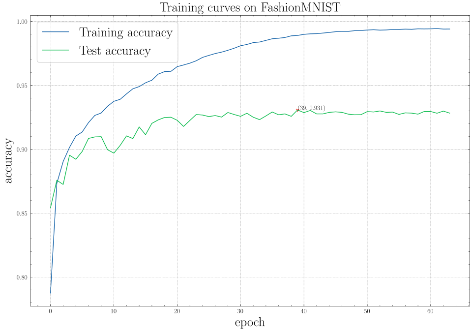
epoch =63, train_loss = 0.0024, train_acc = 0.9941, test_loss = 0.0113, test_acc = 0.9283, max_test_acc = 0.9308
train speed = 7627.8147 images/s, test speed = 7868.9090 images/s
escape time = 2022-05-24 21:42:16
We get max_test_acc = 0.9308. If we fine-tune the hyper-parameters, we will get higher accuracy.
The following figure shows the accuracy curves during training:
Visualizing Encoding#
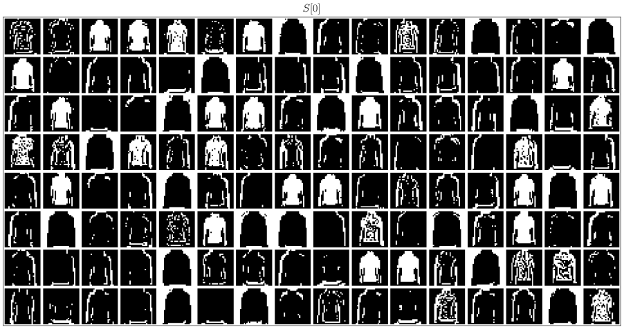
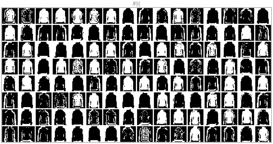
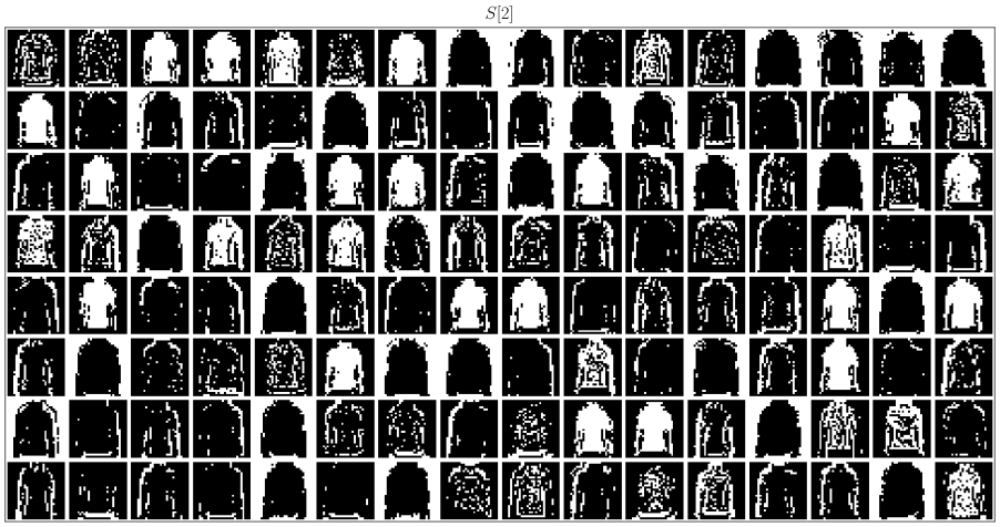
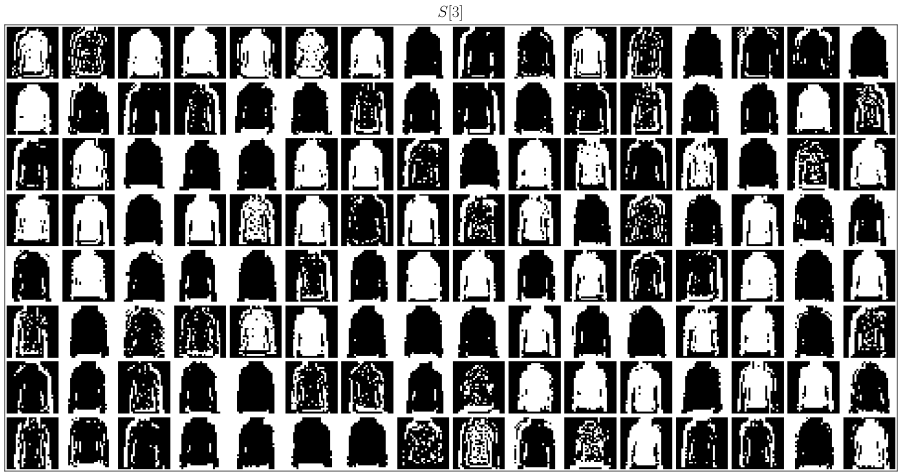
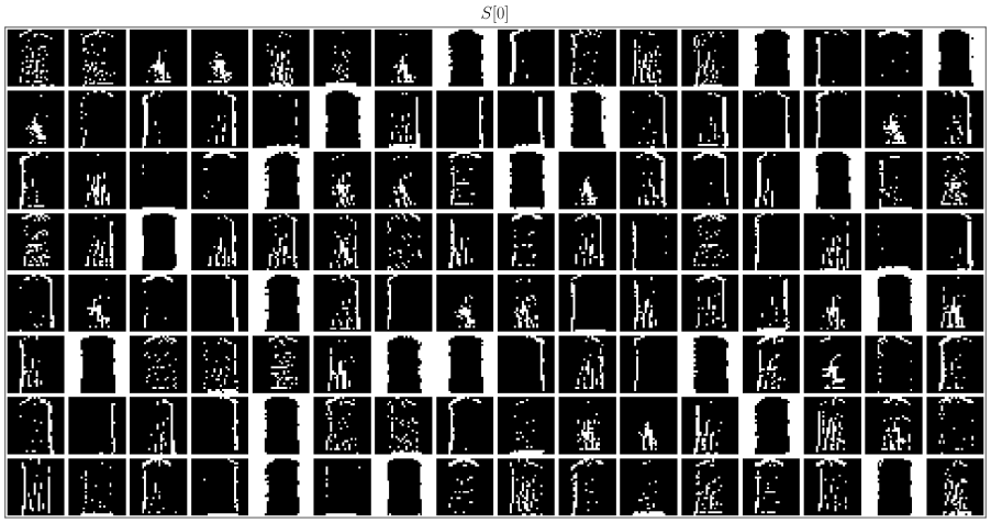
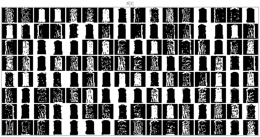
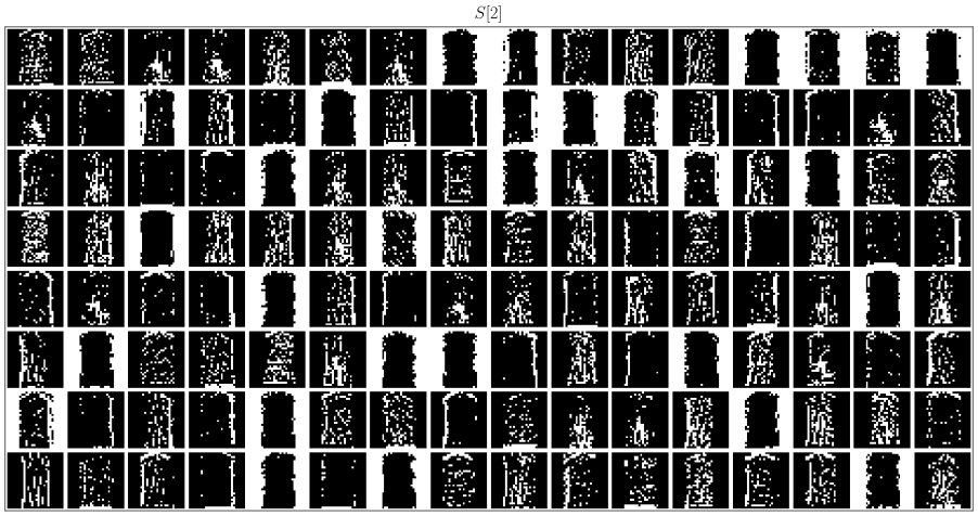
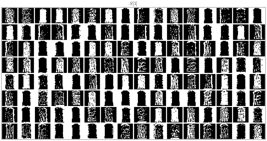
As mentioned above, we send images to SNN directly, and the encoding is implemented by the first {Conv2d-BatchNorm2d-IFNode} in the SNN. Now let us extract the encoder {Conv2d-BatchNorm2d-IFNode}, give images to the encoder, and visualize the output spikes:
# spikingjelly.activation_based.examples.conv_fashion_mnist
class CSNN(nn.Module):
    # ...
    def spiking_encoder(self):
        return self.conv_fc[0:3]
def main():
    # ...
    if args.resume:
        checkpoint = torch.load(args.resume, map_location='cpu')
        net.load_state_dict(checkpoint['net'])
        optimizer.load_state_dict(checkpoint['optimizer'])
        lr_scheduler.load_state_dict(checkpoint['lr_scheduler'])
        start_epoch = checkpoint['epoch'] + 1
        max_test_acc = checkpoint['max_test_acc']
        if args.save_es is not None and args.save_es != '':
            encoder = net.spiking_encoder()
            with torch.no_grad():
                for img, label in test_data_loader:
                    img = img.to(args.device)
                    label = label.to(args.device)
                    # img.shape = [N, C, H, W]
                    img_seq = img.unsqueeze(0).expand(net.T, -1, -1, -1, -1)  # [N, C, H, W] -> [T, N, C, H, W]
                    spike_seq = encoder(img_seq)
                    functional.reset_net(encoder)
                    to_pil_img = torchvision.transforms.ToPILImage()
                    vs_dir = os.path.join(args.save_es, 'visualization')
                    os.mkdir(vs_dir)

                    img = img.cpu()
                    spike_seq = spike_seq.cpu()

                    img = F.interpolate(img, scale_factor=4, mode='bilinear')
                    # 28 * 28 is too small to read. So, we interpolate it to a larger size

                    for i in range(label.shape[0]):
                        vs_dir_i = os.path.join(vs_dir, f'{i}')
                        os.mkdir(vs_dir_i)
                        to_pil_img(img[i]).save(os.path.join(vs_dir_i, f'input.png'))
                        for t in range(net.T):
                            print(f'saving {i}-th sample with t={t}...')
                            # spike_seq.shape = [T, N, C, H, W]

                            visualizing.plot_2d_feature_map(spike_seq[t][i], 8, spike_seq.shape[2] // 8, 2, f'$S[{t}]$')
                            plt.savefig(os.path.join(vs_dir_i, f's_{t}.png'))
                            plt.savefig(os.path.join(vs_dir_i, f's_{t}.pdf'))
                            plt.savefig(os.path.join(vs_dir_i, f's_{t}.svg'))
                            plt.clf()

                    exit()
    # ...
Let us load the trained model, set batch_size=4, which means we only save 4 images and their spikes, and save data in ./logs. The running commands are:
python -m spikingjelly.activation_based.examples.conv_fashion_mnist -T 4 -device cuda:0 -b 4 -epochs 64 -data-dir /datasets/FashionMNIST/ -amp -opt sgd -lr 0.1 -j 8 -resume ./logs/T4_b256_sgd_lr0.1_c128_amp/checkpoint_latest.pth -save-es ./logs
备注
The checkpoint was trained with batch_size=256 (denoted by b256 in the checkpoint path), while the inference command above uses batch_size=4 to save only 4 samples for visualization.
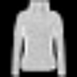
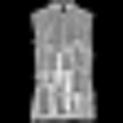
Images and spikes will be saved in ./logs/visualization. Here are two images and spikes encoded from them:
Running the examples and interpreting results#
The model runs on its input device automatically. Reset independent batches
with functional.reset_net after backward and parameter updates; see
Neuron for continuous state. AMP and fused neuron execution are separate
policies. See Training and Inference Precision for state precision and Automatic neuron execution
for compilation and diagnostics.
The accuracy, curves and logs on this page come from historical experiments; some runs lack an exact version. They have not been retrained or verified on current V2, so they cannot establish its speed or accuracy.