Neuron#

This tutorial is about spikingjelly.activation_based.neuron and introduces the spiking neurons.

Spiking Neuron Modules#

In SpikingJelly, we define the spiking neuron as the neuron that can only output spikes (or tensor whose element can only be 0 or 1). The network which uses spiking neurons is the Spiking Neural Network (SNN). Many frequently-used spiking neurons are defined in spikingjelly.activation_based.neuron. Let us use the spikingjelly.activation_based.neuron.IFNode as the example to learn how to use neurons in SpikingJelly.

Firstly, let us import modules:

import torch
from spikingjelly.activation_based import neuron
from spikingjelly import visualizing
from matplotlib import pyplot as plt

Define an IF neurons layer:

if_layer = neuron.IFNode()

There are some parameters for building IF neurons, and we can refer to API docs for more details. For the moment, we just focus on the following parameters:

v_threshold -- threshold of this neurons layer

v_reset -- reset voltage of this neurons layer. If not None, the neuron's voltage will be set to v_reset
after firing a spike. If None, the neuron's voltage will subtract v_threshold after firing a spike

surrogate_function -- the function for calculating surrogate gradients of the heaviside step function in backward

The user may be curious about how many neurons are in this layer. In most of the neurons layer in spikingjelly.activation_based.neuron.IFNode, the number of neurons is defined by the shape of input after this layer is initialized or reset().

Similar to RNN cells, the spiking neuron is stateful (or has memory). The state of spiking neurons is the membrane potentials \(V[t]\). All neurons in spikingjelly.activation_based.neuron have the attribute v. We can print the v:

print(if_layer.v)
# if_layer.v=0.0

We can find that if_layer.v is 0.0 because we have not given the neurons layer any input. Let us give different inputs and check the v.shape. We can find that it is the same with the input:

x = torch.rand(size=[2, 3])
if_layer(x)
print(f'x.shape={x.shape}, if_layer.v.shape={if_layer.v.shape}')
# x.shape=torch.Size([2, 3]), if_layer.v.shape=torch.Size([2, 3])
if_layer.reset()

x = torch.rand(size=[4, 5, 6])
if_layer(x)
print(f'x.shape={x.shape}, if_layer.v.shape={if_layer.v.shape}')
# x.shape=torch.Size([4, 5, 6]), if_layer.v.shape=torch.Size([4, 5, 6])
if_layer.reset()

Note that the spiking neurons are stateful. So, we must call reset() before we give a new input sample to the spiking neurons.

What is the relationship between \(V[t]\) and \(X[t]\)? In spiking neurons, \(V[t]\) is not determined by the input \(X[t]\) at the current time-step t, but also by the membrane potential \(V[t-1]\) at the last time-step t-1.

We use the sub-threshold neuronal dynamics \(\frac{\mathrm{d}V(t)}{\mathrm{d}t} = f(V(t), X(t))\) to describe the charging of continuous-time spiking neurons. For the IF neuron, the charging function is:

\[\frac{\mathrm{d}V(t)}{\mathrm{d}t} = X(t)\]

spikingjelly.activation_based.neuron uses the discrete-time difference equation to approximate the continuous-time ordinary differential equation. The discrete-time difference equation of the IF neuron is:

\[V[t] - V[t-1] = X[t]\]

\(V[t]\) can be got by

\[V[t] = f(V[t-1], X[t]) = V[t-1] + X[t]\]

The equation is written directly in spikingjelly.activation_based.neuron.SimpleIFNode for dynamics experiments:

def neuronal_charge(self, x: torch.Tensor):
    self.v = self.v + x

Different spiking neurons have different charging equations but usually share the firing and reset equations. The spikingjelly.activation_based.neuron.SimpleBaseNode interface expresses these stages directly through the neuronal_charge → neuronal_fire → neuronal_reset path. Production neurons perform the equivalent computation in functional transitions or specialized kernels. The core firing expression in SimpleBaseNode.neuronal_fire is:

def neuronal_fire(self):
    self.spike = self.surrogate_function(self.v - self.v_threshold)

surrogate_function() is the Heaviside step function in forward, which returns 1 when input is greater or equal to 0, otherwise returns 0. We regard the tensor whose element is only 0 or 1 as the spike.

Firing spike will consume the accumulated potential, and make the potential decrease instantly, which is the neuronal reset. In SNN, there are two kinds of reset:

Hard reset: the membrane potential will be set to the reset voltage after firing: \(V[t] = V_{reset}\)
Soft reset: the membrane potential will decrease the threshold potential after firing: \(V[t] = V[t] - V_{threshold}\)

We can find that the neuron that uses soft reset does not need the attribute \(V_{reset}\). In the current implementation of spikingjelly.activation_based.neuron, the default value of v_reset is 0.0, which means the neuron will use hard reset by default.If we set v_reset = None, then the neuron will use the soft reset. SimpleBaseNode.neuronal_reset uses the following equivalent logic:

# The following codes are for tutorials. The actual codes are different but have similar behavior.

def neuronal_reset(self):
    if self.v_reset is None:
        self.v = self.v - self.spike * self.v_threshold
    else:
        self.v = (1. - self.spike) * self.v + self.spike * self.v_reset

Three equations for describing spiking neurons#

Now we can use the three equations: neuronal charge, neuronal fire, and neuronal reset, to describe all kinds of spiking neurons:

\[\begin{split}H[t] & = f(V[t-1], X[t]) \\ S[t] & = \Theta(H[t] - V_{threshold})\end{split}\]

where \(\Theta(x)\) is the surrogate_function in the parameters of __init__. \(\Theta(x)\) is the heaviside step function:

\[\begin{split}\Theta(x) = \begin{cases} 1, & x \geq 0 \\ 0, & x < 0 \end{cases}\end{split}\]

The hard reset equation is:

\[V[t] = H[t] \cdot (1 - S[t]) + V_{reset} \cdot S[t]\]

The soft reset equation is:

\[V[t] = H[t] - V_{threshold} \cdot S[t]\]

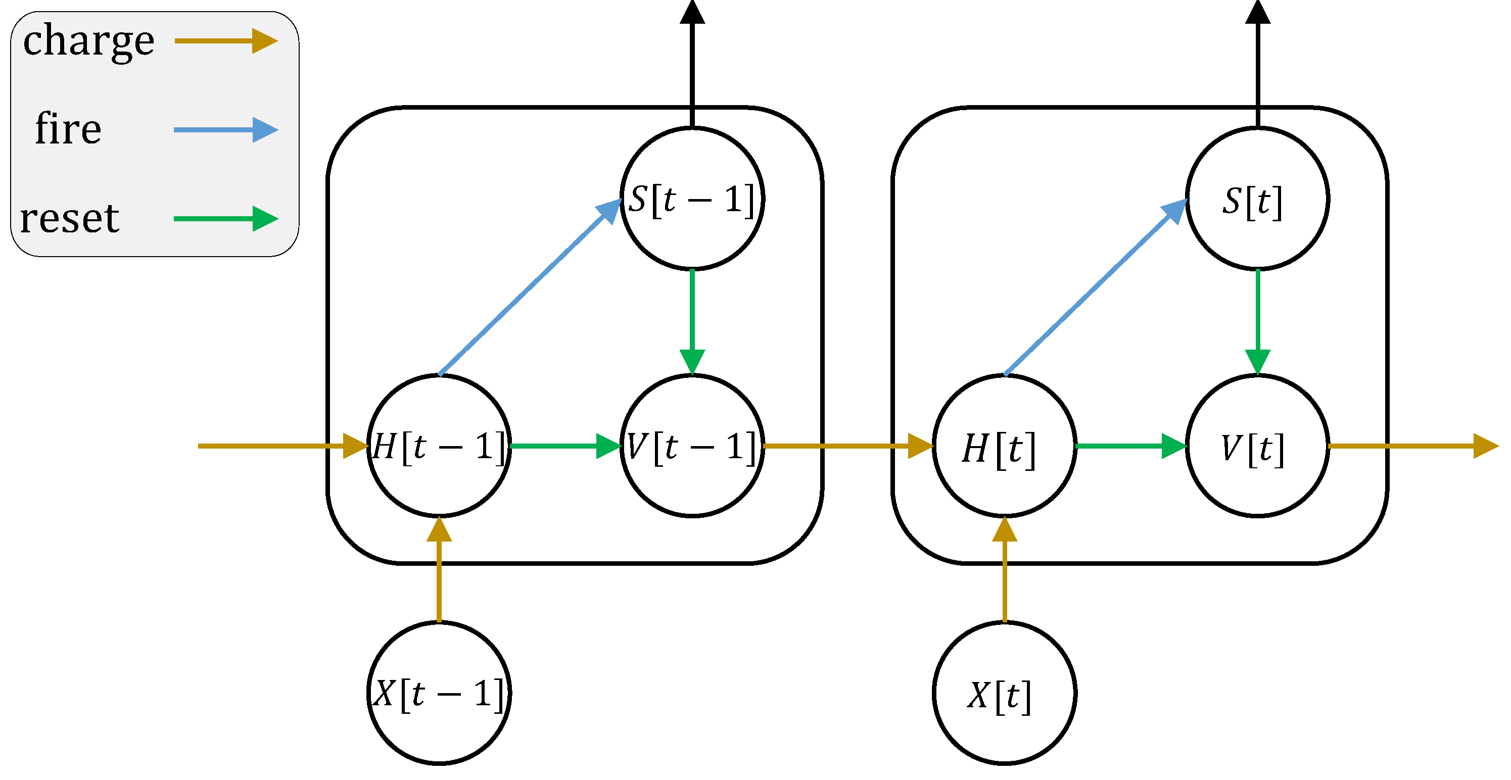
where \(X[t]\) is the external input. To avoid confusion, we use \(H[t]\) to represent the membrane potential after neuronal charging but before neuronal firing. \(V[t]\) is the membrane potential after neuronal firing. \(f(V[t-1], X[t])\) is the neuronal charging function, and is different for different neurons.

The neuronal dynamics can be described by the following figure (the figure is cited from Incorporating Learnable Membrane Time Constant to Enhance Learning of Spiking Neural Networks):

Simulation#

Now let us give inputs to the spiking neurons step-by-step, check the membrane potential and output spikes, and plot them:

if_layer.reset()
x = torch.as_tensor([0.02])
T = 150
s_list = []
v_list = []
for t in range(T):
    s_list.append(if_layer(x))
    v_list.append(if_layer.v)

dpi = 300
figsize = (12, 8)
visualizing.plot_one_neuron_v_s(torch.cat(v_list).numpy(), torch.cat(s_list).numpy(), v_threshold=if_layer.v_threshold,
                                v_reset=if_layer.v_reset,
                                figsize=figsize, dpi=dpi)
plt.show()

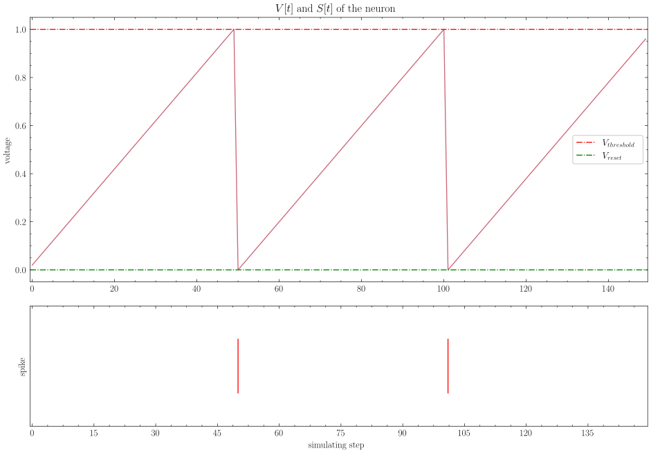
The input has shape=[1]. So, there is only 1 neuron. Its membrane potential and output spikes are:

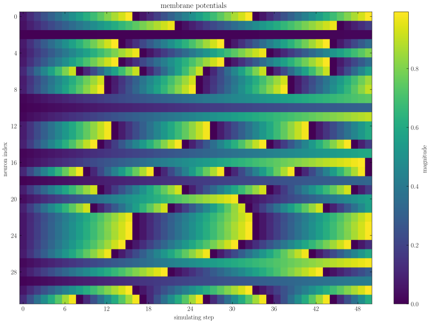
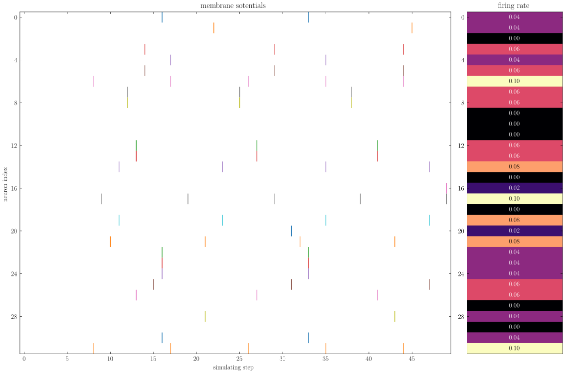
Reset the neurons layer, and give the input with shape=[32]. Then we can check the membrane potential and output spikes of these 32 neurons:

if_layer.reset()
T = 50
x = torch.rand([32]) / 8.
s_list = []
v_list = []
for t in range(T):
    s_list.append(if_layer(x).unsqueeze(0))
    v_list.append(if_layer.v.unsqueeze(0))

s_list = torch.cat(s_list)
v_list = torch.cat(v_list)

figsize = (12, 8)
dpi = 200
visualizing.plot_2d_heatmap(array=v_list.numpy(), title='membrane potentials', xlabel='simulating step',
                            ylabel='neuron index', int_x_ticks=True, x_max=T, figsize=figsize, dpi=dpi)


visualizing.plot_1d_spikes(spikes=s_list.numpy(), title='membrane sotentials', xlabel='simulating step',
                        ylabel='neuron index', figsize=figsize, dpi=dpi)

plt.show()

The results are:

Step mode and backend#

We have introduced step modes in Basic Conception. In the above codes, we use the single-step mode. By setting step_mode, we can switch to multi-step easily:

import torch
from spikingjelly.activation_based import neuron, functional
if_layer = neuron.IFNode(step_mode='s')
T = 8
N = 2
x_seq = torch.rand([T, N])
y_seq = functional.multi_step_forward(x_seq, if_layer)
if_layer.reset()

if_layer.step_mode = 'm'
y_seq = if_layer(x_seq)
if_layer.reset()

Some neurons support the cupy backend in both single-step and multi-step modes. In addition, triton backend is also available for multi-step IFNode, LIFNode, ParametricLIFNode, etc. These accelerated backends can speed up forward and backward.

import torch
from spikingjelly.activation_based import neuron

if_layer = neuron.IFNode()
print(f'if_layer.backend={if_layer.backend}')
# if_layer.backend=torch

print(f'step_mode={if_layer.step_mode}, supported_backends={if_layer.supported_backends}')
# step_mode=s, supported_backends=('torch', 'cupy')

if_layer.step_mode = 'm'
print(f'step_mode={if_layer.step_mode}, supported_backends={if_layer.supported_backends}')
# step_mode=m, supported_backends=('torch', 'cupy', 'triton')

device = 'cuda:0'
if_layer.to(device)
if_layer.backend = 'cupy'  # switch to the cupy backend
print(f'if_layer.backend={if_layer.backend}')
# if_layer.backend=cupy

x_seq = torch.rand([8, 4], device=device)
y_seq = if_layer(x_seq)
if_layer.reset()

if_layer.backend = 'triton'  # switch to the triton backend
print(f'if_layer.backend={if_layer.backend}')
# if_layer.backend=triton

y_seq = if_layer(x_seq)
if_layer.reset()

Custom Spiking Neurons#

SpikingJelly provides separate interfaces for modifying neuron dynamics and for high-performance execution. Simple in SimpleBaseNode describes the role of the interface, not a neuron mathematical model. This pure-PyTorch interface exposes charge, fire, and reset directly so that users can understand the role of a neuron in an SNN and customize its dynamics.

Neuron extension interfaces#
Base class	Forward model	`to_functional_forward`	Intended use
`SimpleBaseNode`	`neuronal_charge` → `neuronal_fire` → `neuronal_reset`	General state-substitution path	Teaching, dynamics experiments, and rapid prototypes
`BaseNode`	Native functional transition with optional sequence kernels	Direct functional-forward call	Production neurons and backend implementations

Inherit from SimpleBaseNode when only the neuron equation needs to change. Its single-step forward always applies charge, fire, and reset in order, and its multi-step forward invokes the complete single-step forward at every time step. Therefore, users normally only implement neuronal_charge. SimpleIFNode and SimpleLIFNode use the same interface.

SimpleBaseNode does not define a native functional transition. Calling functional_forward directly raises an error. Calling to_functional_forward on a module derived from SimpleBaseNode uses the general fallback, which temporarily substitutes explicit registered memories, runs the regular forward, and restores those memories. This preserves the equation extension interface but is less efficient than native-functional neurons such as LIFNode; it is not intended for high-performance workloads that repeatedly require functional conversion.

Production MemoryModule implementations call materialize_states(inputs, states, step_mode) before functional forward. Its default implementation returns states unchanged; override it only when scalar or empty states must become tensors based on the current inputs. inputs contains the complete inputs of the current forward pass. An implementation may use step_mode to select the first time step as its reference in multi-step mode; it must not assume that every input has a time dimension. The method returns a new state tuple and must not mutate module memory. The former BaseNode.v_float_to_tensor hook has been removed.

Suppose we want to build a Square-Integrated-and-Fire neuron, whose neuronal charge equation is:

\[V[t] = f(V[t-1], X[t]) = V[t-1] + X[t]^{2}\]

We can implement this kind of neuron by the following codes:

import torch
from spikingjelly.activation_based import neuron

class SquareIFNode(neuron.SimpleBaseNode):
    def neuronal_charge(self, x: torch.Tensor):
        self.v = self.v + x.square()

Use our SquareIFNode to implement the single/multi-step forward:

import torch
from spikingjelly.activation_based import neuron

class SquareIFNode(neuron.SimpleBaseNode):
    def neuronal_charge(self, x: torch.Tensor):
        self.v = self.v + x.square()

sif_layer = SquareIFNode()

T = 4
N = 1
x_seq = torch.rand([T, N])
print(f'x_seq={x_seq}')

for t in range(T):
    yt = sif_layer(x_seq[t])
    print(f'sif_layer.v[{t}]={sif_layer.v}')

sif_layer.reset()
sif_layer.step_mode = 'm'
y_seq = sif_layer(x_seq)
print(f'y_seq={y_seq}')
sif_layer.reset()

The outputs are:

x_seq=tensor([[0.7452],
        [0.8062],
        [0.6730],
        [0.0942]])
sif_layer.v[0]=tensor([0.5554])
sif_layer.v[1]=tensor([0.])
sif_layer.v[2]=tensor([0.4529])
sif_layer.v[3]=tensor([0.4618])
y_seq=tensor([[0.],
        [1.],
        [0.],
        [0.]])

To implement a production neuron that converts directly like LIFNode and can provide CuPy, Triton, or Inductor kernels, inherit from BaseNode and implement single_step_functional_forward. Its interface is (self, inputs, states, **kwargs) -> (outputs, updated_states). The method must not mutate registered module memories or the supplied states. Override multi_step_functional_forward only when an independent sequence implementation or specialized kernel exists.

警告

Regular BaseNode forward is now functional-backed, and neuronal_charge, neuronal_fire, and neuronal_reset have been removed from it. Existing subclasses that customize Python neuron equations through these methods should change their base class to SimpleBaseNode; their existing equations do not need to be rewritten. Production neurons and custom backends should migrate to the functional interface described above.